Intercomparison of European Fog Forecast Models - Cosmo

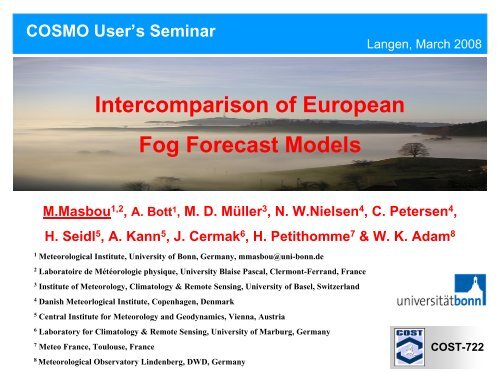
COSMO User’s Seminar
Langen, March 2008
Intercomparison of European
Fog Forecast Models
M.Masbou 1,2 , A. Bott 1 , M. D. Müller 3 , N. W.Nielsen 4 , C. Petersen 4 ,
H. Seidl 5 , A. Kann 5 , J. Cermak 6 , H. Petithomme 7 & W. K. Adam 8
1 Meteorological Institute, University of Bonn, Germany, mmasbou@uni-bonn.de
2 Laboratoire de Météorologie physique, University Blaise Pascal, Clermont-Ferrand, France
3
Institute of Meteorology, Climatology & Remote Sensing, University of Basel, Switzerland
4
Danish Meteorlogical Institute, Copenhagen, Denmark
5
Central Institute for Meteorology and Geodynamics, Vienna, Austria
6
Laboratory for Climatology & Remote Sensing, University of Marburg, Germany
7
Meteo France, Toulouse, France
8
Meteorological Observatory Lindenberg, DWD, Germany
COST-722

Fog Formation
•Cooling
•Moistening
•Turbulent Mixing
1D
3D
Reach saturation
Radiation fog
Advection fog
(1D)
3D
3D
Precipitation fog
Upslope fog
Valley fog

Fog: A visibility reduction
1.4km
1km
0.5 km
100 m
50 m

COST 722 Project
Development of advanced methods for short-range
forecasts of fog, visibility and low clouds
Working Group I: Initial Data
• Improved calibration and analysis of satellite data
• Recommendation of measurement equipments
• Exchange of knowledge and methods
Working Group II: Numerical Models
• Developement of numerical for fog and low clouds
• Improved understanding of physical processes during fog events
Working Group III: Statistical Methods
• Powerful and highly sophisticated statisitcal methods
• Improved expertise on statistical methods
• Basis for the preparation of training material

Comparison Campaign on the Lindenberg Area
September – December 2005
Phase 1: Statistics
Each Participant produce 4 month fog forecast and quantify statistically
his fog forecast quality (FAR, HR, ETS)
Phase 2: Fine Comparison for chosen fog/no fog events
Episode 1: fog formation with mid cloud cover
September, 27th 2005: 01-05 UTC
Episode 2: fog formation with without cloud cover
October, 6th 2005: 07-09 UTC
October, 7th 2005: 06-08 UTC
Episode 3: fog formation with 8/8 cloud cover
December, 6th 2005: 18-00 UTC
December, 7th 2005: 00-23 UTC

Lindenberg Area
Observatory of DWD supplies:
• Visibility 2m
• Cloud cover
• Radiative fluxes
(SW, LW, Latent and Sensible)
• 10m-Mast: T, RH, Wind
• 100m-Mast: T, RH, Wind
• Radiosounding
(00, 06, 12 and 18 UTC)
• Soil temperature
• Soil moisture

Participants
Statistical Model: MOS-ARPEGE
France: H. Petithomme
MOS statistics using linear discriminant analysis
Uses model output of the hydrostatic global model ARPEGE
Predictand:
Predictor:
visibility with different thresholds
pressure at the ground, cloud cover, 10m wind
speed, RH2m, T2m

Model name:
Resolution:
Model domain:
Boundary values:
Dynamics:
Turbulence:
Visibility:
Operational models
Austria: H. Seidl and A. Kann
Model name:
Resolution:
Model domain:
Boundary values:
Dynamics:
Turbulence:
Visibility:
ALADIN-AUSTRIA
9.6 km horizontal, 45 vertical layers
Europe
global model ARPEGE
Hydrostatic
Louis scheme
Post-processing in case of T-inversion
gradient RH and T
Denmark: C. Petersen and N.W. Nielsen
DMI-HIRLAM
16 km horizontal, 40 vertical layers
Europe
ECMWF analyses and forecasts
Hydrostatic
prognostic TKE
MOS approach depending on ground
measurements and model forecasts

Turbulence:
Visibility:
Non-operational models
Germany: M. Masbou and A. Bott
Model name:
LM-PAFOG (COSMO-FOG)
Resolution: 2.8 km horizontal, 40 vertical layers, Δz min =4m
Model domain: 280 x 280 km limited area
Boundary values: COSMO-EU
Dynamics:
Turbulence:
Visibility:
Switzerland: M.D. Müller
Model name:
Resolution:
Model domain:
Boundary values:
Dynamics:
Nonhydrostatic, fully compressible
Louis scheme
diagnostic variable depending on CCN, LWC,
aerosol concentration at 2m
NMM-PAFOG
1 km horizontal, 45 vertical layers
160 x 160 km limited area
NMM 13 km
Nonhydrostatic, fully compressible
prognostic TKE
complex relation of moist forecasted
parameter at 2m

Statistical Study
METHOD
Comparison 1 pixel of Model area with visibility 2m
5 Categories: < 350m, < 600m, < 1000m, < 1500m, < 3000m
Basing on contingence table analyses
PERIOD
4 months forecast (September-December 2005)
MODELS
Initialization:
each day at 00 UTC
FOG CLIMATOLOGY
35 Fog events
Fog episode very rare, 4 % of studied time period

Ensemble Forecast
To analyse the basic quality of the European models
Ensemble forecast extracted from the 4 models
n
1
P = ∑ P
ens
n
i
i=
1
P ens
P i
Fog event probability of the
ensemble
Fog event probability of
the i-th model
n
Quantity of available
forecasts
Average out disagreements
between ensemble member

Hit Rate
What fraction of the observed “fog" events were correctly forecast?
BLACK:LM-PAFOG RED:ENSEMBLE GREEN:HIRLAM
MAGENTA:MOS-ARPEGE
BLUE:ALADIN

False Alarm Rate
What fraction of the observed "no-fog" events were incorrectly forecast as “fog"?
BLACK:LM-PAFOG RED:ENSEMBLE GREEN:HIRLAM
MAGENTA:MOS-ARPEGE
BLUE:ALADIN

False Alarm Ratio
What fraction of the predicted “fog" events actually did not occur
(i.e., were false alarms)?
BLACK:LM-PAFOG RED:ENSEMBLE GREEN:HIRLAM
MAGENTA:MOS-ARPEGE
BLUE:ALADIN

Equitable Threat Score
How well did the forecast “fog" events correspond to the observed “fog" events?
BLACK:LM-PAFOG RED:ENSEMBLE GREEN:HIRLAM
MAGENTA:MOS-ARPEGE
BLUE:ALADIN

Case I: Visibility 2m
Date: September, 26-27 th 2005
After a rain episode bringing warm and humid air, residual cloud
parcel
Radiative fog

Visibility 2m: case I
Legend:
Vis 1000 m
Vis

LWC 2m: case I
Legend:
LWC> 0.1g/kg
>0.01 g/kg
LWC

Case I: Vertical profile at Lindenberg
BLACK:OBSERVED RED:LM-PAFOG GREEN:ALADIN
BLUE:HIRLAM
CYAN= NMM-PAFOG

Case I: Radiative Fluxes

Case I: Close to the ground

Case II: Visibility 2m
Date: December, 6-7 th 2005
Stable moist layer with a tendency to light rain, full cloud cover
Low stratus and Fog

Visibility 2m: case II
Legend:
Vis 1000 m
Vis

LWC 2m: case II
Legend:
LWC> 0.1g/kg
>0.01 g/kg
LWC

Case II: Vertical profile at Lindenberg
BLACK:OBSERVED RED:LM-PAFOG GREEN:ALADIN
BLUE:HIRLAM
CYAN= NMM-PAFOG

Case II: Radiative Fluxes

Case II: Close to the ground

CONCLUSION
4 Models involved NO BEST MODEL
• MOS-ARPEGE: statistic model
• ALADIN-AUSTRIA, DMI-HIRLAM:
3D mesoscale models, ad hoc cloud water near the surface
• NMM-PAFOG, LM-PAFOG :
3D high-resolution fog forecast model, complex microphysics
Statistical and fine Analysis of autumn 2005´s fog events
• 20 % of the fog forecast according with measurements
• Initialization and Assimilation of the boundary layer
determinant role for a successful fog forecast
• Visibility parameterization: decisive key
• Vertical diffusion usually not designed to work well
near the surface

Outlooks
• Adapted turbulent scheme for high vertical resolution
• Long time verification of 3D fog forecast model considering
spatial distribution of fog
• Adjusting the visibility parameterization
Thanks
COST 722

Parameters in Fog Formation
Important Parameters in Fog Formation
Cooling of moist air by radiative flux divergence
Vertical mixing of heat and moisture
Vegetation
Horizontal and vertical wind
Heat and moisture transport in soil
Advection
Topographic effect
(Duynkerke, P.G.,1991)
Once the fog has formed
Longwave radiative cooling at fog top
Gravitational droplet settling
Fog microphysics
Shortwave radiation

What is FOG ?
WMO definition
“Suspension of very small, usually microscopic water
droplets in the air, generally reducing the horizontal
visibility at the Earth´s surface to less than 1km”
Forecaster definition (Roach, W.T., 1994)
“Fog occurs whenever the horizontal visibility falls below
1km. Cloud base descending to ground level is also
experienced as fog.”

Case III: Visibility 2m
Date: October, 6-7 th 2005
Under influence of high pressure system, no cloud cover
Radiative fog

Visibility 2m: case III
Legend:
Vis 1000 m
Vis

LWC 2m: case III
Legend:
LWC> 0.1g/kg
>0.01 g/kg
LWC

Case III: Vertical profile at Lindenberg
BLACK:OBSERVED RED:LM-PAFOG GREEN:ALADIN
BLUE:HIRLAM
CYAN= NMM-PAFOG

Case III: Radiative Fluxes

Case III: Close to the ground