7 Games and Strategies - Luiscabral.net

7 Games and Strategies
Suppose it’s early in 2010. Two major Hollywood studios, Warner Bros. and Fox, are
considering when to release their promising blockbusters targeted at younger audiences:
Warner Bros’ Harry Potter and Fox’s The Chronicles of Narnia. a There are two possibilities:
November or December. Everything else equal, December is a better month; but having
the two movies released at the same time is likely to be bad for both studios.
The dilemma faced by Warner Bros. and Fox illustrates the problem of interdependent
decision making: Warner Bros’ payoff depends not only on its own decision but also on the
decision of another player, Fox. Economists study this type of situations as if Warner Bros.
and Fox were playing a game. b
A game is a stylized model that depicts situations of strategic behavior, where the
payoff for one agent depends on its own actions as well as on the actions of other agents. c
The application of games to economic analysis is not confined to movie release dates. For
example, in a market with a small number of sellers the profits of a given firm depend on
the price set by that firm as well as on the prices set by the other firms. In fact, price
competition with a small number of firms is a typical example of the world of strategic
behavior — and games.
This type of situation introduces a number of important considerations. The optimal
choice for a player — its optimal strategy — depends on what it expects other players will
choose. Since other players act in a similar way, when conjecturing what another player
will do, I may need to conjecture what the other player’s conjecture regarding my behavior
is; and so forth. Moreover, if the strategic interaction evolves over a number of periods,
I should also take into account that my actions today will have an impact on the other
a. Specifically, Harry Potter and the Deathly Hallows: Part I; and The Chronicles of Narnia: The
Voyage of the Dawn Treader.
b. In the U.S., the game resulted in Warner and Fox choosing November 19 and December 10 as release
dates, respectively.
c. Economic analysis is based on the use of models. Models are stylized representations of reality,
highlighting the particular aspects of interest to the economist. Being stylized is not a defect of
models, rather it should be seen as a requisite: a completely realistic model would be as useful as an
exceedingly detailed description of reality, so complete that its main features would be buried in the
abundance of detail. It is helpful to keep this point in mind when judging the very stylized nature of
some of the games and models presented in this text.
Forthcoming in Introduction to Industrial Organization, 2nd Ed. This draft: February 11, 2014.
Cabral.
c○ Luís

players’ beliefs and actions in the future. In summary, payoff interdependence introduces a
host of possibilities for strategic behavior — the object of game theory.
Elements of game theory. The basic element of game theory and applied game theory
is a game. A game consists of a set of players, a set of rules (who can do what when) and a
set of payoff functions (the utility each player gets as a result of each possible combination
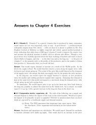
of strategies). Figure 7.1 depicts a simple game which exemplifies these ideas. There are
two players, Player 1 and Player 2. Player 1 has two possible strategies, T and B, which
we represent as Player 1 choosing a row in the matrix represented in Figure 7.1. Player 2
also has two possible strategies, L and R, which we represent by the choice of a column in
the matrix in Figure 7.1.
For each combination of strategies by each player, the respective matrix cell shows the
payoffs received by each player. In the lower left corner, the payoff received by Player 1; in
the top right corner, the payoff received by Player 2. A crucial aspect of a game is that each
player’s payoff is a function of the strategic choice by both players. In Figure 7.1, this is
represented by a matrix, where each cell corresponds to a combination of strategic choices
by each player. This form of representing games is know as normal form. Later we will
consider alternative forms of representing a game.
Simultaneous vs. sequential decisions. One final point regarding the game is Figure
7.1 is the “rule” that both players choose their strategies simultaneously. This rule will be
maintained throughout a number of examples in this chapter — in fact, throughout much of
the book. Therefore, I should clarify its precise meaning. In real life, very seldom do agents
make decisions at precisely the same time. A firm will make a strategic investment decision
this week, its rival will do it in two or three weeks’ time. So how realistic is the assumption
that players choose strategies at the same time? Suppose that there is an observation lag,
that is, suppose that it takes time for Player 2 to observe what Player 1 chooses; and
likewise, suppose that it takes time for Player 1 to observe what Player 2 chooses. In this
context, it is perfectly possible that players make decisions at different times but that, when
decisions are made, neither player knows what the other player’s choice is. In other words,
it is as if players were simultaneously choosing strategies. Naturally, the assumption that
observation lags are very long does not always hold true. Later in the chapter, we will find
examples where an explicit assumption of sequential decision making is more appropriate.
7.1. Nash equilibrium
A game is a model, a stylized description of a real-world situation. The purpose of formulating
such a model is to understand (and predict) behavior patterns, in this case strategic
behavior patterns. In other words, we would like to “solve” the game, that is, determine the
strategies we expect each player to follow. This can be important for descriptive analysis
(understanding why a certain player chooses a certain strategy) as well as for prescriptive
analysis (advising a player what strategy to choose). In this section, I consider various
possible avenues for “solving” a game.
Dominant and dominated strategies. Consider again the game in Figure 7.1. What
strategies would we expect players to choose? Take Player 1’s payoffs, for example. If
2

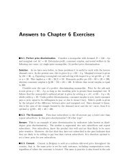
Figure 7.1
The “prisoner’s dilemma” game
Player 1
T
B
5
6
Player 2
L R
5
3
3
4
6
4
Player 1 expects Player 2 to choose L, then Player 1 is better off by choosing B instead of
T . In fact, B would yield a payoff of 6, which is more than the payoff from T , 5. Likewise,
if Player 1 expects Player 2 to choose R, then Player 1 is better off by choosing B instead
of T . In this case, Player 1’s payoffs are given by 3 and 4, respectively. In summary, Player
1’s optimal choice is B, regardless of what Player 2 chooses.
Whenever a player has a strategy that is strictly better than any other strategy regardless
of the other players’ strategy choices, we say that the first player has a dominant strategy.
A dominant strategy yields a player the highest payoff for each and every choice by the
other players.
If a player has a dominant strategy and if the player is rational — that is, payoff maximizing
— then we should expect the player to choose the dominant strategy. Notice that all we
need to assume is that the player is rational. In particular, we do not need to assume that
the other players are rational. In fact, we do not even need to assume the first player knows
the other players’ payoffs. The concept of dominant strategy is very robust.
The structure of the game presented in Figure 7.1 is very common in economics, in
particular in industrial organization. For example, strategies T and L might correspond to
setting a high price, whereas B and R correspond to setting a low price. What is interesting
about this game is that (a) both players are better off by choosing (T, L), which gives each
player a payoff of 5; however, (b) Player 1’s dominant strategy is to play B and Player 2’s
dominant strategy is to play R; (c) For this reason, players chose (B, R) and receive (4,4),
which is less than the commonly beneficial outcome (5,5).
In other words, the game in Figure 7.1, which is commonly known as the prisoner’s
dilemma, depicts the conflict between individual incentives and joint incentives. Jointly,
players would prefer to move from (B, R) to (T, L), boosting payoffs from (4,4) to (5,5).
However, individual incentives are for Player 1 to choose B and for Player 2 to choose
R. In Chapters 8 and 9, we will see that many oligopoly situations have the nature of a
“prisoner’s dilemma.” We will also see in what ways firms can escape the predicament of
lowering payoffs from the “good” outcome (5,5) to the “bad” outcome (4,4).
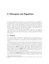
Consider the game in Figure 7.2. There are no dominant strategies in this game. In
fact, more generally, very few games have dominant strategies. We thus need to find other
ways of “solving” the game. Consider Player 1’s decision. While Player 1 has no dominant
strategy, Player 1 has a dominated strategy, namely M. In fact, if Player 2 chooses L,
3

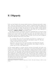
Figure 7.2
Dominated strategies
Player 1
T
M
B
1
0
2
Player 2
L C R
2
0
0
1
0
-2
0
3
1
1
0
2
1
0
2
then Player 1 is better off by choosing T than M. The same is true for the cases when
Player 2 chooses C or R. That is, M is dominated by T from Player 1’s point of view. More
generally,
A dominated strategy yields a player a payoff which lower than that of a different
strategy, regardless of what the other players do.
The idea is that, if a given player has a dominated strategy and that player is rational, then
we should expect that player not to choose such a strategy.
Notice that the definition of a dominated strategy calls for there being another strategy
that dominates the strategy in question. A strategy is not necessarily dominated even if, for
each opponent strategy, we can find an alternative choice yielding a higher payoff. Consider
Figure 7.2 again and suppose that Player 1’s payoff from the (T, R) strategy combination is
−3 instead of 1. Then, for each possible choice by Player 2, we can find a choice by Player
1 that is better than M: if Player 2 chooses L, then T is better than M; if Player 2 chooses
C, then T and B are better than M; and if Player 2 chooses R, then B is better than M.
However, M is not a dominated strategy in this alternative game: there is no other strategy
for Player 1 that guarantees a higher payoff than M regardless of Player 2’s choice.
The concept of dominated strategies has much less “bite” than that of dominant strategies.
If Player 1 has a dominant strategy, we know that a rational Player 1 will choose
that strategy; whereas if Player 1 has a dominated strategy all we know is that it will not
choose that strategy; in principle, there could still be a large number of other strategies
Player 1 might choose. Something more can be said, however, if we successively eliminate
“dominated” strategies. (The justification for quotation marks around “dominated” will
soon become clear.)
Suppose that Player 2 knows Player 1’s payoffs and, moreover, knows that Player 1 is
rational. By the reasoning presented earlier, Player 2 should expect Player 1 not to choose
M. Given that Player 1 does not choose M, Player 2 finds strategy C to be “dominated”
by R. Notice that, strictly speaking, C is not a dominated strategy: if Player 1 chooses M
then C is better than R. However, C is dominated by R given that M is not played by
Player 1.
We can now take this process one step further. If Player 1 is rational, believes that
4

Figure 7.3
Dubious application of dominated strategies
Player 2
L R
Player 1
T
B
0
1 1
0
-100 2
1
1
Player 2 is rational, and believes that Player 2 believes that Player 1 is rational, then
Player 1 should find T to be a “dominated” strategy (in addition to M). In fact, if Player
2 does not choose C, then strategy T is “dominated” by strategy B: if Player 2 chooses
L, Player 1 is better off with B; if Player 2 chooses R, again, Player 1 is better off with
B. Finally, if we take this process one step further, we conclude that L is a “dominated”
strategy for Player 2. This leaves us with the pair of strategies (B, R).
As in the first example, we have reached a single pair of strategies, a “solution” to
the game. However, the assumptions necessary for iterated elimination of “dominated”
strategies to work are much more stringent than in the case of dominant strategies. Whereas
in the first example all we needed to assume was that players are rational, payoff maximizing
agents, we now assume that each player believes that the other player is rational.
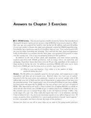
To understand the importance of these assumptions regarding rationality, consider the
simple game in Figure 7.3. Player 2 has a dominated strategy, L. In fact, it has a dominant
strategy, too (R). If Player 1 believes that Player 2 is rational, then Player 1 should expect
Player 2 to avoid L and instead play R. Given this belief, Player 1’s optimal strategy is to
play B, for a payoff of 2. Suppose, however, that Player 1 entertains the possibility, unlikely
as it might be, that Player 2 is not rational. Then B may no longer be its optimal choice,
since there is a chance of Player 2 choosing L, resulting in a payoff of −100 for Player 1. A
more general point is that, in analyzing games,
It is not only important whether players are rational: it is also important whether
players believe the other players are rational.
Absolute and relative payoff. The game in Figure 7.3 also raises the issue of what
rationality really means. In game theory, we take it to imply that players seek to maximize
their payoff. However, many students, faced with the game in Figure 7.3, expect Player 2
to choose L: while it implies a lower payoff for Player 2 (0 instead of 1) it also gives Player
1 a very negative payoff. In other words, the outcome (B, L) looks favorable to Player 2 in
the sense that Player 2 “wins” by a very favorable margin. Given that Player 1 chooses B,
Player 2 would get a greater payoff by choosing L, but it would “lose” to Player 1, in the
sense that it would receive a lower payoff than Player 1.
Although this is a frequent interpretation of games like that in Figure 7.3, in differs
from the game theory approach. Instead, we assume that each rational player’s goal is to
5

Figure 7.4
A game with no dominant or dominated strategies
Player 2
L C R
T
2
1 2
0 0
3
Player 1
M
1
1 1
1 1
0
B
0
1 0
2 2
2
maximize his or her payoff. It is quite possible that one component of a player’s payoff is
the success (or lack thereof) of rival players. If that is the case, then we should include it
explicitly as part of the player’s payoff. For example, suppose that the values in Figure 7.3
correspond to monetary payoffs; and that each player’s payoff is equal to the cash payoff
plus a relative performance component computed as follows: earning one extra dollar more
than the rival is equivalent to earning 10 cents in cash. Then the relevant game payoffs,
given that Player 1 chooses B, would be (−110, +10) (if Player 2 chooses L) and (2.1, 0.9)
(if Player 2 chooses R). d
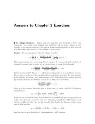
Nash equilibrium. Consider now the game in Figure 7.4. There are no dominant or
dominated strategies in this game. Is there anything we can say about what to expect
players will choose? In this game, more than in the previous games, it is apparent that each
player’s optimal strategy depends on what the other player chooses. We must therefore
propose a conjecture by Player 1 about Player 2’s strategy and a conjecture by Player
2 about Player 1’s strategy. A natural candidate for a “solution” to the game is then a
situation whereby (a) players choose an optimal strategy given their conjectures of what
the other players do and (b) such conjectures are consistent with the other players’ strategy
choice.
Suppose that Player 1 conjectures that Player 2 chooses R; and that Player 2 conjectures
that Player 1 chooses B. Given these conjectures, Player 1’s optimal strategy is B, whereas
Player 2’s optimal strategy is R. In fact, if Player 1 conjectures that Player 2 chooses R,
then B is Player 1’s optimal choice; any other choice would yield a lower payoff. The same
if true for Player 2. Notice that, based on these strategies, the players’ conjectures are
consistent: Player 1 expects Player 2 to choose what in fact Player 2 finds to be an optimal
strategy, and vice-versa. This situation is referred to as a Nash equilibrium. 1
Although the concept of Nash equilibrium can be defined with respect to conjectures,
it is simpler — and more common — to define it with respect to strategies.
d. It would follow in this case that R is no longer a dominant strategy for Player 2 and as a result that
Player 1 is better off by choosing T .
6

Figure 7.5
Best responses
Player 2’s
strategy
L
C
R
Player 1’s
strategy
T
Player 1’s
best response
T
B
B
Player 2’s
best response
R
M {L,C }
B
R
Player 1
T
M
B
Player 2
L C R
1 2
2 ∗ 0
1
0
1 ∗
1
1
1 ∗
0
1
3 ∗
0
0 2 ∗
2 ∗ 2 ∗
A pair of strategies constitutes a Nash equilibrium if no player can unilaterally change
its strategy in a way that improves its payoff.
It can be checked that, in the game in Figure 7.4, (B, R) is a Nash equilibrium and no
other combination of strategies is a Nash equilibrium. For example, (M, C) is not a Nash
equilibrium because, given that Player 2 chooses C, Player 1 would rather choose T .
Best responses. A useful way to find a game’s Nash equilibrium is to derive each
player’s best response. Player 1’s best response is a mapping that indicates Player 1’s best
strategy for each possible strategy by Player 2. The left panels in Figure 7.5 shows Player
1’s (top) and Player 2’s (bottom) best-response mapping. For example, if Player 2 chooses
L, then Player 1 gets 2 from playing T , 1 from playing M, and 0 from playing B. It follows
that Player 1’s best response to Player 2 choosing L is given by T ; and so forth. Regarding
Player 2’s best response, notice that, if Player 1 chooses M, then L and C all are equally
good choices for Player 2 (and better than R). For this reason, Player 2’s best response
corresponds to the set {L, C}.
How are best responses related to Nash equilibrium? Let BR 1 (s 2 ) and BR 2 (s 1 ) be Player
1’s and Player 2’s best response mappings, respectively. A Nash equilibrium is then a pair
of strategies s ∗ 1 and s∗ 2 such that s∗ 1 is the best response to s∗ 2 and vice-versa. Continuing
with the game described in Figure 7.4, a helpful way of representing these best response
mappings is to go back to the game matrix and mark with an asterisk (or some other
symbol) the payoff values corresponding to a best response. This is done in the matrix on
the right-hand side of Figure 7.5. A Nash equilibrium then corresponds to a cell where both
payoffs are marked with an asterisk. As can be seen from Figure 7.5, in our example this
corresponds to the pair of strategies (B, R) — which confirms our previous finding.
Continuous variables. In this introductory chapter, I only consider games where players
chose among a finite number of possible actions and strategies. However, consider a gas
station’s pricing strategy. There are many different values of price it can choose from. If
7

Figure 7.6
Multiple Nash equilibria
Player 2
L R
Player 1
T
B
1
0
2
0
0
2
0
1
we assume only a few possible values — for example, $2, $3 and $4 per gallon — we may
artificially limit the player’s choices. If instead we assume each and every possible price
to the cent of the dollar, then we end up with enormous matrices.
In situations like this, the best solution is to model the player’s strategy as picking a
number from a continuous set. This may be too unrealistic in that it allows for values that
are not observed in reality (for example, selling gasoline at $ √ 2 per gallon). However, it
delivers a better balance between realism and tractability.
Suppose that player i chooses a strategy x i (for example, a price level) from some set S
(possibly a continuous set). Player i’s payoff is a function of its choice as well as its rival’s:
π i (x i , x j ). In this context, a pair of strategies (x ∗ i , x∗ j ) constitutes a Nash equilibrium if
and only if, for each player i, there exists no strategy x ′ i such that π i(x ′ i , x∗ j ) > π i(x ∗ i , x∗ j ).
An equivalent definition may be given in terms of best response mappings. Let BR i (x j )
be player i’s best response to player j’s choice. Then a Nash equilibrium is a pair of
strategies (x ∗ i , x∗ j ) such that, for each player i, x∗ i = BR i(x ∗ j ).
In Chapter 8 we will use this methodology for determining the equilibrium of some
oligopoly games.
Multiple equilibria and focal points. Contrary to the choice of dominant strategies,
application of the Nash equilibrium concept always produces an equilibrium. e In fact, there
may exist more than one Nash equilibrium. One example of this is given by the game in
Figure 7.6, where both (T, L) and (B, R) are Nash equilibria. A possible illustration for
this game is the process of standardization. Strategies T and L, or B and R, correspond
to combinations of strategies that lead to compatibility. Both players are better off under
compatibility. However, Player 1 prefers compatibility around the standard (B-R), whereas
Player 2 prefers compatibility over the other standard. More generally, this example is
representative of a class of games in which (a) players want to coordinate, (b) there is more
than one point of coordination, (c) players disagree over which of the two coordination
points in better. f
Equilibrium multiplicity can be problematic for an analyst: if the game’s equilibrium
is a natural prediction of what will happen when players interact, then multiplicity makes
e. For the sake of rigor, two qualifications are in order: First, existence of Nash equilibrium applies to
most games but not to all. Second, equilibria sometimes require players to randomly choose one of
the actions (mixed strategies), whereas we have only considered the case when one action is chosen
with certainty (pure strategies).
f. Standardization problems are further discussed in Chapter 18.
8

such prediction difficult. This is particularly the case for games that have not only two but
many different equilibria. Consider the following example: two people are asked to choose
independently and without communication where and when in New York City they would
try to meet one another. If they choose the same meeting location then they both receive
$100; otherwise they both receive nothing. 2 Despite the plethora of possible meeting and
time locations, which correspond to a plethora of Nash equilibria, a majority of subjects
typically choose Grand Central Station at noon: the most salient traffic hub in New York
City and the most salient time of the day.
Although there is an uncountable number of Nash equilibria in the “meet me in New
York” game, some are more “reasonable” than others. Here, “reasonable” is not meant
in the game theoretic sense: all equilibria satisfy the conditions for a Nash equilibrium.
Rather, it is meant in the sense that, based on information that goes beyond the game
itself, there may be focal points on which players coordinate even if they do not communicate.
g Game theory and the concept of Nash equilibrium are useful tools to understand
interdependent decision-making; but they are not the only source of useful information to
predict equilibrium behavior.
7.2. Sequential games h
In the previous section, we justified the choice of simultaneous-choice games as a realistic
way of modeling situations where observation lags are so long that it is as if players were
choosing strategies simultaneously. When the time between strategy choices is sufficiently
long, however, the assumption of sequential decision making is more realistic. Consider the
example of an industry that is currently monopolized. A second firm must decide whether
or not to enter the industry. Given the decision of whether or not to enter, the incumbent
firm must decide whether to price aggressively or not. The incumbent’s decision is taken
as a function of the entrant’s decision. That is, first the incumbent observes whether or
not the entrant enters, and then decides whether or not to price aggressively. In such a
situation, it makes more sense to consider a model with sequential rather than simultaneous
choices. Specifically, the model should have the entrant — Player 1 — move first and the
incumbent — Player 2 — move second.
The best way to model games with sequential choices is to use a game tree. A game
tree is like a decision tree only that there is more than one decision maker involved. An
example is given by Figure 7.7, where strategies and payoffs illustrate the case of entrant
and incumbent described above. In Figure 7.7, a square denotes a decision node. The game
starts with decision node 1. At this node, Player 1 (entrant) makes a choice between e and
ē, which can be interpreted as “enter” and “not enter,” respectively. If the latter is chosen,
then the game ends with payoffs π 1 = 0 (entrant’s payoff) and π 2 = 50 (incumbent’s payoff).
If Player 1 chooses e, however, then we move on to decision node 2. This node corresponds
to Player 2 (incumbent) making a choice between r and ¯r, which can be interpreted as
“retaliate entry” or “not retaliate entry,” respectively. Games which, like Figure 7.7, are
g. One game theorist defined a focal point as “each person’s expectation of what the other expects him
to expect to be expected to do.”
h. This and the next section cover relatively more advanced material which may be skipped in a first
reading of the book.
9

Figure 7.7
Extensive-form representation: the sequential-entry game
1
ē
e
.
0, 50
¯r
.
2
r
.
.
10, 20
-10, 10
represented by trees are also referred to as games in extensive form. i
This game has two Nash equilibria: (e, ¯r) and (ē, r). Let us first check that (e, ¯r) is
indeed a Nash equilibrium, that is, no player has an incentive to change its strategy given
what the other player does. First, if Player 1 chooses e, then Player 2’s best choice is to
choose ¯r (it gets 20, it would get −10 otherwise). Likewise, given that Player 2 chooses ¯r,
Player 1’s optimal choice is e (it gets 10, it would get 0 otherwise).
Let us now check that (ē, r) is an equilibrium. Given that Player 2 chooses r, Player 1
is better off by choosing ē: this yields Player 1 a payoff of 0, whereas e would yield −10.
As for Player 2, given that Player 1 chooses ē, its payoff is 50, regardless of which strategy
it chooses. It follows that r is an optimal choice (though not the only one).
Although the two solutions are indeed two Nash equilibria, the second equilibrium does
not make much sense. Player 1 is not entering because of the “threat” that Player 2 will
choose to retaliate. But, is this threat credible? If Player 1 were to enter, would Player 2
decide to retaliate? Clearly, the answer is “no”: by retaliating, Player 2 gets −10, compared
to 20 from no retaliation. We conclude that (ē, r), while being a Nash equilibrium, is not a
reasonable prediction of what one might expect to be played out.
One way of getting rid of this sort of “unreasonable” equilibria is to solve the game
backward; that is, to apply the principle of backward induction. First, we consider node
2, and conclude that the optimal decision is ¯r. Then, we solve for the decision in node 1
given the decision previously found for node 2. Given that Player 2 will choose ¯r, it is now
clear that the optimal decision at node 1 is e. We thus select the first Nash equilibrium as
the only that is intuitively “reasonable.”
Solving a game backward is not always this easy. Suppose that, if Player 1 chooses e
at decision node 1 we are led not to a Player 2 decision node but rather to an entire new
game, say, a simultaneous-move game as in Figures 7.1 to 7.6. Since this game is a part
of the larger game, we call it a subgame of the larger game. In this setting, solving the
game backward would amount to first solving for the Nash equilibrium (or equilibria) of
the subgame; and then, given the solution for the subgame, solving for the entire game.
Equilibria which are derived in this way are called subgame-perfect equilibria. 3 For simple
game trees like the one in Figure 7.7, subgame-perfect equilibria are obtained by solving
the game backwards, that is, backwards induction and subgame perfection coincide.
i. From this and the previous sections, one might erroneously conclude that games with simultaneous
choices must be represented in the normal form and games with sequential moves in the extensive
form. In fact, both simultaneous and sequential choice games can be represented in both the normal
and extensive forms. However, for simple games like those considered in this chapter, the choice of
game representation considered in the text is the more appropriate.
10

Figure 7.8
The value of commitment
2
¯b
b
.
1
.
1
ē
e
ē
e
.
.
0, 50
¯r
.
2
r
0, 50
¯r
.
2
r
.
.
.
.
10, 20
-10, -10
10, -20
-10, -10
The value of credible commitment. In the game of Figure 7.7, the equilibrium (ē, r)
was dismissed on the basis that it requires Player 2 to make the “incredible” commitment of
playing r in case Player 1 chooses e. Such threat is not credible because, given that Player
1 has chosen e, Player 2’s best choice is ¯r. But suppose that Player 2 writes an enforceable
and not renegotiable contract whereby, if Player 1 chooses e, then Player 2 must choose r.
The contract is such that, were Player 2 not to choose r and choose ¯r instead, Player 2
would incur a penalty of 40, lowering its total payoff to −20. j
The situation is illustrated in Figure 7.8. The first decision now belongs to Player 2, who
must choose between writing the bond described above (strategy b) and not doing anything
(strategy ¯b). If Player 2 chooses ¯b, then the game in Figure 7.7 is played. If instead Player
2 chooses b, then a different game is played, one that takes into account the implications of
issuing the bond.
Let us now compare the two subgames starting at Player 1’s decision nodes. The one
on top is the same as in Figure 7.7. As we then saw, restricting to the subgame perfect
equilibrium, Player 2’s payoff is 20. The subgame on the bottom is identical to the one on
top except for Player 2’s payoff following (e, r). The value is now −20 instead of 20. At
first, it might seem that this makes Player 2 worse off: payoffs are the same in all cases
except one; and in that one case payoff is actually lower than initially. However, as we will
see next, Player 2 is better off playing the bottom subgame than the top one.
Let us solve the bottom subgame backward, as before. When it comes to Player 2 to
choose between r and ¯r, the optimal choice is r. In fact, this gives Player 2 a payoff of
−10, whereas the alternative would yield −20 (Player 2 would have to pay for breaking the
bond). Given that Player 2 chooses r, Player 1 finds it optimal to choose ē: it is better
to receive a payoff of zero than to receive −10, the outcome of e followed by r. In sum,
the subgame on the bottom gives Player 2 an equilibrium payoff of 50, the result of the
combination ē and r.
We can finally move backward one more stage and look at Player 2’s choice between b
j. This is a very strong assumption as most contracts are renegotiable. However, for the purposes of
the present argument, what is important is that Player 2 has the option of imposing on itself a cost
if it does not choose r. This cost may result from breach of contract or from a different cause.
11

Figure 7.9
Modeling Player 2’s capacity to precommit
2
¯r
r
.
1
.
1
ē
e
ē
e
.
.
.
.
0, 50
10, 20
0, 50
-10, -10
and ¯b. From what we saw above, Player 2’s optimal choice is to choose b and eventually
receive a payoff of 50. The alternative, ¯b, eventually leads to a payoff of 20 only.
This example illustrates two important points. First it shows that
A credible commitment may have significant strategic value.
By signing a bond that imposes a large penalty when playing ¯r, Player 2 credibly commits
to playing r when the time comes to choose between r and ¯r. In so doing, Player 2 induces
Player 1 to choose ē, which in turn works in Player 2’s benefit. Specifically, introducing
this credible commitment raises Player 2’s payoff from 20 to 50. Therefore, the value of
commitment in this example is 30.
The second point illustrated by the example is a methodological one. If we believe
that Player 2 is credibly committed to choosing r, then we should model this by changing
Player 2’s payoffs or by changing the order of moves. This can be done as in Figure 7.8,
where we model all the moves that lead to Player 2 effectively precommiting to playing r.
Alternatively, this can also be done as in Figure 7.9, where we model Player 2 as choosing
r or ¯r “before” Player 1 chooses its strategy. The actual choice of r or ¯r may occur in time
after Player 1 chooses e or ē. However, if Player 2 precommits to playing r, we can model
that by assuming Player 2 moves first. In fact, by solving the game in Figure 7.9 backward,
we get the same solution as in Figure 7.8, namely the second Nash equilibrium of the game
initially considered.
Short-run and long-run. To conclude this section, we should mention another instance
where the sequence of moves plays an important role. This is when the game under consideration
depicts a long-term situation where players choose both long-run and short-run
variables. For example, capacity decisions are normally a firm’s long-term choice, for production
capacity (buildings, machines) typically lasts for a number of years. Pricing, on the
other hand, is typically a short-run variable, for firms can change it relatively frequently at
a relatively low cost.
When modeling this sort of strategic interaction, we should assume that players choose
the long-run variable first and the short-run variable second. Short-run variables are those
that players choose given the value of the long-run variables. And this is precisely what we
12

Figure 7.10
A game with long-run and short-run strategy choices: timing of moves
Players 1 and 2 choose
long term variable
.
Players 1 and 2 choose
short term variable
.
get by placing the short-run choice in the second stage.
This timing of moves is depicted in Figure 7.10. This figure illustrates yet a third
way of representing games: a time-line of moves. This is not as complete and rigorous as
the normal-form and extensive-form representations we saw before; but it proves useful in
analyzing a variety of games.
In a real-world situation, as time moves on, firms alternate between choosing capacity
levels and choosing prices, the latter more frequently than the former. If we want to
model this in a simple, two-stage game, then the right way of doing it is to place the
capacity decision in the first stage and the pricing decision in the second stage. The same
principle applies more generally when there are long-run and short-run strategic variables.
In the following chapters, we will encounter examples of this in relation to capacity/pricing
decisions (Chapter 8), product positioning/pricing decisions (Chapter 15), and entry/output
decisions (Chapter 11).
7.3. Repeated games
Many real-world situations of strategic behavior are repeated over an extended period of
time. Sometimes, this can be modeled by an appropriate static model. For example, in the
previous section we saw how a two-stage game can be used to model competition in longterm
and short-term variables. Consider, however, the strategic phenomenon of retaliation,
that is, the situation whereby a player changes its action in response to a rival’s action.
Clearly, this cannot be achieved in a static, simultaneous-move game, for in such game there
is no time for a player to react to another player’s actions.
A useful way to model the situation whereby players react to each other’s moves is to
consider a repeated game. Consider a simultaneous-choice game like the one in Figure 7.1.
Since in this game each player chooses one action only once, we refer to it as a one-shot
game. A repeated game is defined by a one-shot game — also referred to as stage game
— which is repeated a number of times. If repetition takes place a finite number of times,
then we have a finitely repeated game, otherwise we have an infinitely repeated game.
In one-shot games, strategies are easy to define. In fact, strategies are identified with
actions. In repeated games, however, it is useful to distinguish between actions and strategies.
Consider again the game depicted in Figure 7.1, a version of the “prisoner’s dilemma.”
As we saw earlier, it is a dominant strategy for Player 1 to choose B and it is a dominant
strategy for Player 2 to choose R; the unique Nash equilibrium thus implies a payoff of 4
for each player.
Now suppose that this one-shot game is repeated indefinitely. Specifically, suppose that,
after each period actions are chosen and payoffs distributed, the game ends with probability
1 − δ. For simplicity, suppose that players assign the same weight to payoffs earned in any
period. Now the set of strategies is different from the set of actions available to players in
13

each period. In each period, Player 1 must choose an action from the set {T, B}, whereas
Player 2 must choose an action from the set {L, R}; these sets are the players’ action sets.
Strategies, however, can be rather complex combinations of “if-then” statements where the
choice at time t is made dependent on what happened in previous periods; in other words,
strategies can be history dependent. Given the conditional nature of strategies, the number
of strategies available to a player is considerably greater than the number of actions it can
choose from (cf Exercise 7.13).
Specifically, consider the following strategies for Players 1 and 2: if in the past Player 1
chose T and Player 2 chose L, then continue doing so in the current period. If at any time
in the past either of the players made a different choice, then let Player 1 choose B and
Player 2 choose R in the current period.
Can such a pair of strategies form a Nash equilibrium? Let us first compute the equilibrium
payoff that Player 1 gets playing the equilibrium strategies. Recall that (T, L) induces
a payoff of 5 for Player 1. Total expected payoff is therefore given by
V = 5 + δ 5 + δ 2 5 + ... = 5
1 − δ
Notice that I successively multiply payoffs by δ for this is the probability that the game
will continue on. Now consider the possibility of deviating from the equilibrium strategies.
If at a given period Player chooses B instead of T , then expected payoff is given by
V ′ = 6 + δ 4 + δ 2 4 + ... = 6 +
4 δ
1 − δ
In order for the proposed set of strategies to be a Nash equilibrium, it must be that V ≥ V ′ ,
that is
5
1 − δ ≥ 6 + 4 δ
1 − δ
which is equivalent to δ ≥ 1 2
. Given the symmetry of the payoff function, the computations
for Player 2 are identical to those of Player 1. We thus conclude that, if the probability that
the game ends continues on into the next period, δ, is sufficiently high, then there exists a
Nash equilibrium whereby players pick T in every period (while the game is still going on).
Intuitively, the difference between the one-shot game and the indefinitely repeated game
is that, in the latter, we can create a system of inter-temporal rewards and punishments that
induces the right incentives for players to choose T . In one-shot play, the temptation for
Player 1 to play B is too high: it is a dominant strategy, it yields a higher payoff regardless
of what the other player does. In repeated play, however, the short-term gain achieved by
choosing B must be balanced against the different continuation payoff each choice induces.
The equilibrium strategies are such that, if Player 1 chooses B in the current period, then it
gets 4 in every subsequent period. We thus have a gain of 1 in the short run (6 − 5) against
a loss of 1 in every future period (5 − 4). Whether future periods matter or not depends on
the value of δ. If δ is very high then the loss of 1 in every future period counts very heavily,
and Player 1 prefers to stick to T and forego the short-term gain from choosing B.
We conclude that
Because players can react to other players’ past actions, repeated games allow for
equilibrium outcomes that would not be an equilibrium in the corresponding one-shot
game.
14

As we will see in Chapter 9, this idea of “agreements” between players that are enforced by
mutual retaliation plays an important role in explaining the working of cartels and, more
generally, the nature of collusive behavior.
To conclude, a note on concepts and terminology. There are two different interpretations
for the role played by the parameter δ introduced earlier. One is that the game will
end in finite time but the precise date when it will end is unknown to players; all they know
is that, after each period, the game ends with probability 1 − δ. This is the interpretation
I considered in this section and corresponds to the term indefinitely-repeated game. An
alternative interpretation is that the game lasts for an infinite number of periods and that
players discount future payoffs according to the discount factor δ: a dollar next period
is worth δ dollars in the current period. This is the interpretation corresponding to the
term infinitely-repeated game. Formally, the two interpretations lead to the same equilibrium
computation. I prefer the indefinitely-repeated game interpretation and terminology.
However, it is rarely used.
7.4. Information
Consider the pricing dilemma faced by a health insurance company: a low price leads to
small margins, but a high price runs the risk of attracting only high-risk patients. What
should the insurance company do? Specifically, consider the following sequential game
between an insurance company and a patient. First the insurance company decides whether
to charge a high premium or a low premium; then, the patient decides whether or not to
accept the company’s offer.
So far, this looks like a sequential game like the ones considered in Section 7.2. But now
we add a twist: the patient may either be a low-risk patient or a high-risk patient; moreover,
the patient knows what type he is but the insurance company does not. Specifically, the
insurance company believes that with probability 10% the patient is a high-risk patient. For
a high-risk patient, health insurance is worth $20k a year, whereas for a low-risk patient,
the value is $3k. For the insurance company, the cost of providing insurance is $30k for a
high-risk patient and $1k for a low-risk patient.
Notice that, based on the prior probabilities that the patient is high or low risk, the
insurer estimates that the average valuation is given by 10% × 20 + 90% × 3 = 4.7, whereas
the average cost of insuring a patient is given by 10% × 30 + 90% × 1 = 3.9. Based on these
average, the insurance company is considering two possible prices: $4.5k (a price that is
below average valuation but above average cost) or $30 (a price that covers cost regardless
of patient type). k
How do we model this situation as a game? First, notice that, to the extent that actions
are sequential, it will be easiest to model the interaction between insurer and patient
based on a game tree (as I did in Section 7.2). One important difference with respect to
the basic sequential games considered earlier is that we now have uncertainty to consider:
specifically, the patient may be high risk (probability 10%) or low risk (probability 90%).
Moreover, insurer and patient are differently informed regarding risk: specifically, we consider
the extreme case where the patient knows exactly his type but the insurer only has
prior probabilistic beliefs.
k. Below I consider other possibilities.
15

Figure 7.11
Sequential game with asymmetric information
I
-25.5
.
−25.5 × 10% + 0 × 90% = PH
= −2.5
high risk (10%)
.
N
low risk (90%)
.
PL
3.5
0
.
PH
high risk (10%)
.
N
low risk (90%)
0 =
= 0 × 10% + 0 × 90%
.
PL
0
p = 4.5
p = 30
buy
don’t buy
buy
don’t buy
buy
don’t buy
buy
don’t buy
.
.
.
.
.
.
.
.
-25.5, 15.5
0, 0
3.5, -1.5
0, 0
0, -10
0, 0
29, -27
0, 0
In order to model games where there is uncertainty and asymmetric information, we
introduce a new “player” into the game; we call this player Nature. Nature is not a player
like other players: it has no strategic motives and its actions are limited to choosing different
branches of a game tree according to pre-determined probabilities. This may seem a bit
strange, but the example we are considering may help clarify things.
Figure 7.11 shows the game tree for the insurer-patient game. First, the insurer must
decided whether to set a price of 4.5 or 30. Regardless of what the insurer chooses, the next
move is by Nature, which “decides” whether the patient is high risk or low risk according
to the probabilities considered earlier. Finally, given the insurer’s choice as well as Nature’s
choice, the patient either accepts or rejects the insurer’s offer. For ease of reading the tree,
I use two different names for the patient, depending on his type: P H or P L for high-risk
or low-risk patient, respectively.
As in Section 7.2, I proceed by solving the game backwards. If p = 4.5, then the patient
accepts the offer if he is high risk but rejects the offer if he is low risk If p = 30, in turn,
then neither a high-risk patient nor a low-risk patient accept the offer.
Moving back one step, we compute the expected value for player I given Nature’s move:
If p = 4.5, then I’s expected payoff is given by −25.5 × 10% + 0 × 90% = −2.5; if p = 30,
then expected payoff is simply 0. Finally, given these expected payoffs we can solve for I’s
optimal strategy, which is p = 30.
In sum, equilibrium strategies are as follows: the insurer chooses p = 30; the patient
accepts the offer p = 4.5 if he is high risk and rejects the offer if p = 4.5 and he is low risk
or if p = 30 (regardless of risk type).
There are a lot of interesting economics regarding this game, but for now I will focus
on the game theory elements. First, we model uncertainty by creating the player Nature.
16

Figure 7.12
Sequential game with uncertainty but no asymmetric information
I
p = 4.5
p = 30
[0.6,0.2]
.
P
.
P
[0,0]
[0.6,0.2]
.
N
buy
don’t buy
.
N
[0,0]
[0,0]
.
N
buy
don’t buy
.
N
[26.1,-25.3]
hr (10%)
lr (90%)
hr (10%)
lr (90%)
hr (10%)
lr (90%)
hr (10%)
lr (90%)
.
.
.
.
.
.
.
.
-25.5, 15.5
3.5,-1.5
0, 0
0, 0
0, -10
29, -27
0, 0
0, 0
Second, we model asymmetric information by placing the informed player’s nodes after Nature’s
move and the uninformed player’s nodes before Nature’s move. This is an important
modeling choice. Consider an alternative possibility: neither the insurer nor the patient
himself know the level of risk; all they know is the prior probabilities, namely that the
probability of being high risk is 10%. Figure 7.12 depicts the tree corresponding to this
alternative game. Now the order of moves is different: first, I choses the price; next, P
decides whether or not to accept the offer; and finally, N determines whether P is high or
low risk.
Solving the game backwards, we see that the equilibrium corresponds to: I offers a price
p = 4.5; P accepts a p = 4.5 offer but rejects a p = 30 offer (and nature chooses patient type
as before). This is a very different outcome than in the game considered in Figure 7.11. As
we saw in Section 7.2, the order of moves matters, namely when commitment matters; we
now have one additional reason why the order of moves is important: if Nature is involved,
then changing the order of moves changes the nature of information, that is, who knows
what when.
Standard games with asymmetric information. The game between insurer and patient
corresponds to a typical situation of asymmetric information, namely the case when an
uninformed player (e.g., an insurer) must make a move (e.g., offer insurance policy terms)
before the informed player (e.g., the patient) gets to make its move (e.g., accept or reject
the offer). The equilibrium of such games typically involves what economists refer to as
adverse selection. Let us go back to the game in Figure 7.11. By setting a low price,
p = 4.5 the insurer offers a deal that is acceptable for an average patient. However, no
patient is average: in practice, low-risk patients turn down the offer and all the insurer gets
17

is high-risk patients, in which cases revenues fail to cover cost.
There are many real-world examples that feature adverse selection. For example, a
buyer who makes an offer for a used car should take into account that the offer will only
be accepted by sellers who own cars of poor quality (which they know better than the
buyer). On a lighter note, in Groucho Marx’s autobiography we learn that, in response
to an acceptance letter from a club, “I sent the club a wire stating, ‘PLEASE ACCEPT MY
RESIGNATION. I DON’T WANT TO BELONG TO ANY CLUB THAT WILL ACCEPT PEOPLE LIKE
ME AS A MEMBER’.” Can you see why Groucho was playing an adverse selection game?
How does club membership related to health insurance?
As I mentioned earlier, adverse selection results from models where the uninformed party
makes the first move. Consider now the opposite case, that is, the case when the informed
party makes the first move. As a motivating example, think of a firm that enters the market
for luxury luggage. The firm would like to reduce price to gain market share, but worries
that this might be interpreted by customers as a sign of low quality. The key word here is
“signal.” In fact, asymmetric information games where the informed party moves first are
frequently referred to as signaling games. In Chapter 13 I discuss a particularly important
signaling game: the reputation building game, where a player’s actions in the first period
indirectly provide information about his type, which in turn has an effect on how the game
is played in the second period. In Chapter 16 I consider a different application of the same
principles and develop a model of advertising as a signal of quality.
Finally, the principal-agent problem provides an additional example of a game with
asymmetric information. Consider the case of an employer who wants to encourage his
sales team to work hard but cannot observe whether or not they are doing all they can.
What steps can he take to ensure that they work hard? A similar problem occurs in the
relation between a board of directors and a firm’s manager (cf Chapter 3). Still another
example is given by the relation between a regulator and a regulated firm (cf Chapter 5).
What these examples have in common is a principal (employer, shareholder, regulator)
who would like to induce some kind of good behavior from an agent (employee, manager,
regulated utility) but cannot directly observe the agent’s actions or the agent’s type. In the
former case, known as moral hazard (or hidden action) the agent has better information
only with respect to the action that he takes and that the principal does not observe. The
key in games of moral hazard is that even though the principal might not observe the agent’s
actions, she might be able to observe outcomes that are related to actions (for example,
output, an observable, is a function of effort, an unobservable). Then the principal might
want to set up a reward system based on observables—though she should beware about
exactly what kind of behavior this encourages.
Summary
• A dominant strategy yields a player the highest payoff for each and every choice by the
other players. • A dominated strategy yields a player a payoff which lower than that of a
different strategy, regardless of what the other players do. • It is not only important whether
players are rational: it is also important whether players believe the other players are
rational. • A pair of strategies constitutes a Nash equilibrium if no player can unilaterally
18

change its strategy in a way that improves its payoff. • A credible commitment may
have significant strategic value. • Because players can react to other players’ past actions,
repeated games allow for equilibrium outcomes that would not be an equilibrium in the
corresponding one-shot game.
Key concepts
• game • normal form • dominant strategy • prisoner’s dilemma • dominated
strategy • Nash equilibrium • best response • focal points • game tree
• decision node • extensive form • backward induction • subgame
• subgame-perfect equilibria • credible commitment • retaliation • one-shot
game • repeated game • stage game • uncertainty • asymmetric information
• Nature • adverse selection • signaling games • principal-agent • moral
hazard
Review and practice exercises
7.1. Dominant and dominated strategies. What are the assumptions regarding player
rationality implicit in solving a game by elimination of dominated strategies? Contrast this
with the case of dominant strategies.
7.2. The movie release game. Consider the example at the beginning of the chapter.
Suppose that there are only two blockbusters jockeying for position: Warner Bros.’s Harry
Porter and Fox’s Narnia. Suppose that blockbusters released in November share a total of
$500 million in ticket revenues, whereas blockbusters released in December share a total of
$800 million.
(a) Formulate the game played by Warner Bros. and Fox.
(b) Determine the game’s Nash equilibrium(a).
7.3. Ericsson v Nokia. Suppose that Ericsson and Nokia are the two primary competitors
in the market for 4G handsets. Each firm must decide between possible price levels: $100
and $90. Production cost is $40 per handset. Firm demand is as follows: if both firms price
at 100, then Nokia sells 500, Ericsson 800; if both firms price at 90, then sales are 800 and
900, respectively; if Nokia prices at 100 and Ericsson at 90, then Nokia’s sales drop to 400,
whereas Ericsson’s increase to 1100; finally, if Nokia prices at 90 and Ericsson at 100 then
19

Nokia sells 900, Ericsson 700.
(a) Suppose firms choose prices simultaneously. Describe the game and
solve it.
(b) Suppose that Ericsson has a limited capacity of 800k units per quarter.
Moreover, all of the demand unfulfilled by Ericsson is transferred to
Nokia. How would the analysis change?
(c) Suppose you work for Nokia. Your Chief Intelligence Officer (CIO) is
unsure whether Ericsson is capacity constrained or not. How much
would you value this piece of info?
7.4. ET. In the movie “E.T.,” a trail of Reese’s Pieces, one of Hershey’s chocolate brands,
is used to lure the little alien out of the woods. As a result of the publicity created by this
scene, sales of Reese’s Pieces trebled, allowing Hershey to catch up with rival Mars.
Universal Studio’s original plan was to use a trail of Mars’ M&Ms. However, Mars
turned down the offer, presumably because it thought $1m was a very high price. The
makers of “E.T.” then turned to Hershey, who accepted the deal.
Suppose that the publicity generated by having M&Ms included in the movie would
increase Mars’ profits by $800,000 and decrease Hershey’s by $100,000. Suppose moreover
that Hershey’s increase in market share costs Mars a loss of $500,000. Finally, let b be the
benefit for Hershey’s from having its brand be the chosen one.
Describe the above events as a game in extensive form. Determine the equilibrium as a
function of b. If the equilibrium differs from the actual events, how do you think they can
be reconciled?
7.5. ET (reprise). Return to Exercise 7.4. Suppose now that Mars does not know the
value of b, believing that either b =$1,200,000 or b =$700,000, each with probability 50%.
Unlike Mars, Hershey knows the value of b. Draw the tree for this new game and determine
its equilibrium.
7.6. Hernan Cortéz. Hernan Cortz, the Spanish navigator and explorer, is said to have
burnt his ships upon arrival to Mexico. By so doing, he effectively eliminated the option
of him and his soldiers returning to their homeland. Discuss the strategic value of this
action knowing the Spanish colonists were faced with potential resistance from the Mexican
natives.
7.7. HDTV standards. Consider the following game depicting the process of standard
setting in high-definition television (HDTV). 4 The U.S. and Japan must simultaneously
decide whether to invest a high or a low value into HDTV research. If both countries
choose a low effort than payoffs are (4,3) for U.S. and Japan, respectively; if the U.S.
chooses a low level and Japan a high level, then payoff are (2,4); if, by contrast, the U.S.
chooses a high level and Japan a low one, then payoffs are (3,2). Finally, if both countries
20

choose a high level, then payoff are (1,1).
(a) Are there any dominant strategies in this game? What is the Nash
equilibrium of the game? What are the rationality assumptions implicit
in this equilibrium?
(b) Suppose now the U.S. has the option of committing to a strategy
ahead of Japan’s decision. How would you model this new situation?
What are the Nash equilibria of this new game?
(c) Comparing the answers to (a) and (b), what can you say about the
value of commitment for the U.S.?
(d) “When pre-commitment has a strategic value, the player that makes
that commitment ends up ‘regretting’ its actions, in the sense that,
given the rivals’ choices, it could achieve a higher payoff by choosing
a different action.” In light of your answer to (b), how would you
comment this statement?
7.8. Finitely repeated game. Consider a one-shot game with two equilibria and suppose
this game is repeated twice. Explain in words why there may be equilibria in the two-period
game which are different from the equilibria of the one-shot game.
7.9. American Express’s spinoff of Shearson. In 1993, American Express sold Shearson
to Primerica (now part of Citigroup). In the March 9 Wall Street Journal: “Among the
sticking points in acquiring Shearson’s brokerage operations would be the firm’s litigation
costs. More than most brokerage firms, Shearson has been socked with big legal claims
by investors who say they were mistreated, though the firm has made strides in cleaning
up its backlog of investor cases. In 1992’s fourth quarter alone, Shearson took reserves of
$90 million before taxes for ’additional legal provisions.”’ When the deal was completed,
Primerica bought most of Shearson’s assets but left the legal liabilities with American
Express. Why do you think the deal was structured this way? Was it fair to American
Express?
7.10. Sale of business. Suppose that a firm owns a business unit that it wants to
sell. Potential buyers know that the seller values the unit at either $100m, $110m, $120,
. . . $190m, each value equally likely. The seller knows the precise value, but the buyer
only knows the distribution. The buyer expects to gain from synergies with its existing
businesses, so that its value is equal to seller’s value plus $10m. (In other words, there are
gains from trade.) Finally, the buyer must make take-it-or-leave-it offer at some price p.
How much should the buyer offer?
Challenging exercises
7.11. Ad games. Two firms must simultaneously choose their advertising budget.
Suppose payoffs are given by the values in the table below.
Firm 2
21

Figure 7.13
Stage game
Player 2
L C R
T
5
5
3
6
0
0
Player 1
M
6
3
4
4
0
0
B
0
0
0
0
1
1
L
H
Firm 1
L
H
5
8
5
1
1
4
8
4
(a) Determine the Nash equilibria of the one-shot game.
(b) Suppose the game is indefinitely repeated and that the relevant discount
factor is δ = .8. Determine the optimal symmetric equilibrium.
(c) (challenge question) Now suppose that, for the first 10 periods, firm
payoffs are twice the values represented in the above table. What is
the optimal symmetric equilibrium?
7.12. Finitely repeated game I. Suppose that the game depicted in Figure 7.1 is repeated
T times, where T is known. Show that the only subgame perfect equilibrium is for players
to choose B in every period.
7.13. Finitely repeated game II. Consider the game depicted in Figure 7.13. l
(a) Determine the set of Nash equilibrium of the game where choices are
made once.
(b) Suppose that the matrix game in Figure 7.13 is played twice. How
many different strategies does a player now have?
(c) Show that there exists a subgame perfect Nash equilibrium such that
(T, L) is played in the first period.
(d) Compare your answers to the previous questions and comment.
l. This game is identical to that in Figure 7.1 except that we add a third strategy to each player. While
this third strategy leads to an extra Nash equilibrium, the main feature of the game in Figure 7.1
is still valid — namely, the conflict between individual and joint incentives that characterizes the
“prisoner’s dilemma.”
22

7.14. Centipede. Consider the game below. 5 Show, by backward induction, that rational
players choose d at every node of the game, yielding a payoff of 2 for Player 1 and zero for
Player 2. Is this equilibrium reasonable? What are the rationality assumptions implicit in
it?
[
r r r r r
. . . . . . . . r r r
. . . .
1 2 1 2 1 2 1 2
. . . . . . . .
d d d d d d d d
.
2
0
] [
.
1
3
] [
.
4
2
] [
.
3
5
] [
.
6
4
] [
.
97
99
] [
.
100
98
] [
.
99
101
]
[
100
100
]
7.15. Advertising levels. Consider an industry where price competition is not very
important: all of the action is on advertising budgets. Specifically, total value S (in dollars)
gets splits between two competitors according to their advertising shares. If a 1 is firm 1’s
advertising investment (in dollars), then its profit is given by
a 1
a 1 + a 2
S − a 1
(The same applies for firm 2). Both a 1 and a 2 must be non-negative. If both firms invest
zero in advertising, then they split the market.
(a) Determine the symmetric Nash equilibrium of the game whereby firms
choose a i independently and simultaneously.
(b) Determine the jointly optimal level of advertising, that is, the level a ∗
that maximizes joint profits.
(c) Given that firm 2 sets a 2 = a ∗ , determine firm 1’s optimal advertising
level.
(d) Suppose that firms compete indefinitely in each period t = 1, 2, ..., and
that the discount factor is given by δ ∈ [0, 1]. Determine the lowest
value of δ such that, by playing grim strategies, firms can sustain an
agreement to set a ∗ in each period.
23

Endnotes
1. Nash, John (1951), “Non-Cooperative Games,” Annals of Mathematics 54, 286–295.
2. A version of this experiment was first reported in Schelling, Thomas (1960), The Strategy of Conflict,
Cambridge, MA: Harvard University Press
3. Selten, Reinhard (1965), “Spieltheoretische Behandlung eines Oligopolmodells mit Nachfragetragheit,”
Zeitschrift für die gesamte Staatswissenschaft 121, 301–324, 667–689.
4. This exercise is adapted from Dixit, Avinash K., and Barry J. Nalebuff (1991), Thinking Strategically, New
York: W W Norton.
5. This game was first proposed by Rosenthal, Robert (1981), “Games of Perfect Information, Predatory Pricing
and the Chain-Store Paradox,” Journal of Economic Theory 25, 92–100.
24