8 Oligopoly - Luiscabral.net

8 Oligopoly
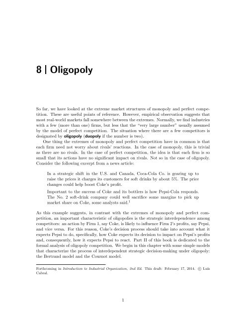
So far, we have looked at the extreme market structures of monopoly and perfect competition.
These are useful points of reference. However, empirical observation suggests that
most real-world markets fall somewhere between the extremes. Normally, we find industries
with a few (more than one) firms, but less that the “very large number” usually assumed
by the model of perfect competition. The situation where there are a few competitors is
designated by oligopoly (duopoly if the number is two).
One thing the extremes of monopoly and perfect competition have in common is that
each firm need not worry about rivals’ reactions. In the case of monopoly, this is trivial
as there are no rivals. In the case of perfect competition, the idea is that each firm is so
small that its actions have no significant impact on rivals. Not so in the case of oligopoly.
Consider the following excerpt from a news article:
In a strategic shift in the U.S. and Canada, Coca-Cola Co. is gearing up to
raise the prices it charges its customers for soft drinks by about 5%. The price
changes could help boost Coke’s profit.
Important to the success of Coke and its bottlers is how Pepsi-Cola responds.
The No. 2 soft-drink company could well sacrifice some margins to pick up
market share on Coke, some analysts said. 1
As this example suggests, in contrast with the extremes of monopoly and perfect competition,
an important characteristic of oligopolies is the strategic interdependence among
competitors: an action by Firm 1, say Coke, is likely to influence Firm 2’s profits, say Pepsi,
and vice versa. For this reason, Coke’s decision process should take into account what it
expects Pepsi to do, specifically, how Coke expects its decision to impact on Pepsi’s profits
and, consequently, how it expects Pepsi to react. Part II of this book is dedicated to the
formal analysis of oligopoly competition. We begin in this chapter with some simple models
that characterize the process of interdependent strategic decision-making under oligopoly:
the Bertrand model and the Cournot model.
Forthcoming in Introduction to Industrial Organization, 2nd Ed. This draft: February 17, 2014.
Cabral.
c○ Luís
1

8.1. The Bertrand model
Pricing is probably the most basic strategy that firms must decide on. The demand received
by each firm depends on the price it sets. Moreover, when the number of firms is small,
demand also depends on the prices set by rival firms. It is precisely this interdependence between
rivals’ decisions that differentiates duopoly competition (and more generally oligopoly
competition) from the extremes of monopoly and perfect competition. When Lenovo, for
example, decides what prices to set for its PCs, the company has to make some conjecture
regarding the prices set by rival Dell; and based on this conjecture determine the optimal
price, taking into account how demand for the Lenovo PC depends on both the Lenovo
price and the Dell price. a
In order to analyze the interdependence of pricing decisions, we begin with the simplest
model of duopoly competition: the Bertrand model. 2 The model consists of two firms in a
market for a homogeneous product and the assumption that firms simultaneously set prices.
We also assume that both firms have the same constant marginal cost, MC = c. b
Since the duopolists’ products are perfect substitutes (the product is homogeneous), and
since firms have no capacity constraint, it follows that whichever firm sets the lowest price
gets all of the demand. Specifically, if p i , the price set by firm i, is lower than p j , the price
set by firm j, then firm i’s demand is given by D(p i ) (the market demand), whereas firm
j’s demand is zero. If both firms set the same price, p i = p j = p, then each firm receives
one half of market demand, 1 2 D(p).
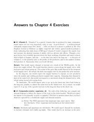
The discrete Bertrand game. Let us first consider the case when sellers are restricted to
a limited set of price levels. Specifically, suppose that market demand is given by q = 10−p,
marginal cost constant at 2, and sellers can only set integer values of price: 3, 4 and
5. Figure 8.1 describes the game in normal form (similarly to the games introduced in
Chapter 7): Firm 1 chooses a row (5, 4 or 3), whereas Firm 2 chooses a column (5, 4 or
3). For each possible combination, profits are determined according to the rules described
in the preceding paragraph. For example, if both firms set p = 5, then total demand is
q = 10 − 5 = 5; and each firm’s profit is given by π = 1 2
5 (5 − 2) = 7.5. If Firm 1 sets
p 1 = 4 whereas Firm 2 sets p 2 = 5, then Firm 1 captures all of the market demand, which
is now given by q = 10 − 4 = 6. It follows that π 1 = 6 (4 − 2) = 12, whereas π 2 = 0. The
remaining cells of the game matrix are obtained in a similar manner. (Check this.)
What is the game’s equilibrium? First notice that there is no dominant strategy. I can
however derive each firm’s best response and from this derive the game’s Nash equilibrium.
Firm 1’s best response mapping is as follows: if Firm 2 sets p 2 = 5, then Firm 1’s optimal
price is p 1 = 4; if Firm 2 sets p 2 = 4, then Firm 1’s optimal price is p 1 = 3; and finally, if
Firm 2 sets p 2 = 3 then Firm 1’s optimal price is p 1 = 3. In words, Firm 1’s best response
is to undercut Firm 2 — unless Firm 2 is already setting the lowest price. As a result, the
Nash equilibrium corresponds to both firms setting the lowest price: ̂p 1 = ̂p 2 = 3.
Notice that, while the game is not, strictly speaking, a a prisoner’s dilemma, it does
share some of the features of the prisoner’s dilemma game (cf Chapter 7). Specifically, (a)
a. Moreover, in a dynamic setting, Lenovo must also take into account that current price choices will
likely influence the rival’s future price choices. This we will see in Chapter 9.
b. The Bertrand model is more general than the simplified version presented here, but the main ideas
are the same.

Figure 8.1
Bertrand game with limited number of price choices
Firm 1
5
4
3
Firm 2
5 4 3
7.5 12 7
7.5 0 0
0 6 7
12 6 0
0 0 3.5
7 7 3.5
both firms are better off by setting a high price; (b) however, given that both firms set a
high price, both firms have an incentive to undercut the rival.
The above game is based on a number of simplifying assumptions. In particular, I am
restricting firms to set prices at integer values (3, 4 or 5). What if Firm 1 could undercut
p 2 = 5 by setting p 1 = 4.99? In the next paragraphs, I consider the more general case when
firms can set any value of p i , in fact any real value. As we will see, the main qualitative
results and intuition remain valid. In fact, in some sense the result will be even more
extreme.
The continuous case. Suppose now that firms can set any value of p from 0 to +∞,
including non-integer values. Now we are unable to describe the game as a matrix of
strategies (there are infinitely many strategies). However, we can derive, as before, each
firm’s best response mapping, from which we can then derive the Nash equilibrium. Recall
that firm i’s best response p ∗ i (p j) is a mapping that gives, for each price by firm j, firm i’s
optimal price. The only novelty with respect to the discrete case is that the values of p j
and p i now vary continuously.
Suppose that Firm 1 expects Firm 2 to price above monopoly price. Then Firm 1’s
optimal strategy is to price at the monopoly level. In fact, by doing so Firm 1 gets all of the
demand and receives monopoly profits (the maximum possible profits). If Firm 1 expects
Firm 2 to price below monopoly price but above marginal cost, then Firm 1’s optimal
strategy is to set a price just below Firm 2’s: c pricing above would lead to zero demand
and zero profits; and pricing below gives firm i all of the market demand, but lower profits
the lower the price is. Finally, if Firm 1 expects Firm 2 to price below marginal cost, then
Firm 1 optimal choice is to price higher than Firm 2, say, at marginal cost level.
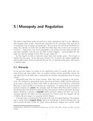
Figure 8.2 depicts Firm 1’s best response, p ∗ 1 (p 2), in a graph with each firm’s strategy
on each axis. Consistent with the above derivation, for values of p 2 less than MC , Firm 1
chooses p 1 = MC = c. For values of p 2 greater than MC but lower than p M , Firm 1 chooses
p 1 just below p 2 . Finally, for values of p 2 greater than monopoly price, p M , Firm 1 chooses
c. What does “just below” mean? If p 1 could be any real number, than “just below” would not be well
defined: there exists no real number “just below” another real number. In practice, prices have to
be set on a finite grid (in cents of the dollar, for example), in which case “just below” would mean
one cent less. This points to an important assumption of the Bertrand model: Firm 1 will steal all
of Firm 2’s demand even if its price is only one cent lower than the rival’s.

Figure 8.2
Bertrand model: best responses and equilibrium.
p ∗ 2(p 1 )
p ∗ 1(p 2 )
̂p 1 = c
N
•
p 1
... ... ... . . .... ... ... ... .. .... ... .... ... ... ... ... . ............
p 2
̂p 2 = c
p 1 = p M .
Since Firm 2 has the same marginal cost as Firm 1, its best response is identical to Firm
1’s, that is, symmetric with respect to the 45 ◦ line. In Figure 8.2, Firm 2’s best response is
given by p ∗ 2 (p 1).
As we saw in Chapter 7, a Nash equilibrium is a pair of strategies — a pair of prices,
in the present case — such that no firm can increase profits by unilaterally changing price.
In terms of Figure 8.2, this is given by the intersection of the best responses, that is, point
N. In fact this is the point at which p 1 = p ∗ 1 (p 2) (because the point is on Firm 1’s best
response) and p 2 = p ∗ 2 (p 1) (because the point is on Firm 2’s best response). As can be seen
from Figure 8.2, point N corresponds to both firms setting a price equal to marginal cost,
̂p 1 = ̂p 2 = MC = c.
Another way of deriving the same conclusion is to think about a possible equilibrium
price p ′ greater than marginal cost. If both firms were to set that price, each would earn
1
2 D(p′ )(p ′ − MC ). However, but setting a slightly smaller price, one of the firms would be
able to almost double its profits to D(p ′ − ɛ)(p ′ − ɛ − MC ), where ɛ is a small number. This
argument holds for any possible candidate equilibrium price p ′ greater than marginal cost.
We thus conclude that the only possible equilibrium price is p = c. In summary,
Under price competition with homogeneous product and constant, symmetric marginal
cost (Bertrand competition), firms price at the level of marginal cost.
Notice that this result is valid even with only two competitors (as we have considered
above). This is a fairly drastic result: as the number of competitors changes from one
to two, equilibrium price changes from monopoly price to perfect competition price. Two
competitors are sufficient to guarantee perfect competition.
From a consumer welfare point of view, Bertrand competition is a tremendous boon.
From the seller’s point of view, however, it is a rather unattractive situation: the Bertrand
trap, as some call it. Consider for example the case of encyclopedias. 4 Encyclopedia Bri-

Box 8.1. Digital yellow pages: from monopoly to duopoly to oligopoly. 3
In 1987, Nynex began offering in digital form the entire telephone directory for the
area the company then served (New York and New England). With a list price of
$10,000, the CD product was primarily targeted at retailers, government departments
and financial service operators.
Soon after, Jim Bryant, the Nynex executive in charge of developing the new Nynex
product, decided to leave the company and found Pro CD, a company devoted to
publishing white and yellow page directories in electronic form.
Fearing competition, Nynex declined to offer the required data for Pro CD to compile
his listing. Undeterred by this obstacle, Bryant sent physical copies of the directories
to Asia, where he outsourced the task of typing them from scratch (and retyping, to
check for errors). All in all, Pro CD created a mega-directory with more than 70 million
entries.
Facing competition in the market for electronic directories, Nynex was forced to lower
its price. By the early 1990s, sale prices were in the hundreds of dollars, down from the
original $10,000 price tag. Meanwhile, additional entrants joined Pro CD in challenging
Nynex’s initial monopoly. By 2000, a complete directory could be bought for a mere
$20. e
tannica has been, for more than two centuries, a standard reference work. Until the 1990s,
the thirty-two-volume hardback set sold for $1,600. Then Microsoft entered the market
with Encarta, which it sold on CD for less than $100. Britannica responded by issuing its
own CD version as well. By 2000, both Britannica and Encarta were selling for $89.99.
While this is still far from the Bertrand equilibrium (price equal to the cost of the CDs)
it is certainly closer to Bertrand than the initial, monopoly-like price of $1,600. Box 8.1
describes another example of how even one competitor can drive prices down tremendously.
Avoiding the Bertrand trap. There are many real-world markets where the number of
firms is small — two or a few more —, firms compete on price, and still firm profits are
positive — sometimes very large. (Can you think of some?) This seems to contradict
the Bertrand model’s prediction. How can we explain this apparent contradiction between
theory and empirical observation? Put differently: if you consult with a firm competing
in a price-setting duopoly, how do you help your client avoid the Bertrand trap? In what
follows, I consider four different solutions, two which I will develop in later chapters, two of
which I will cover in the remainder of this section.
1. Product differentiation. The Bertrand model assumes that both firms sell the same
product. If instead firms sell differentiated products, then duopoly price competition
does not necessarily drive prices down to marginal cost as predicted by the Bertrand
model. In fact, undercutting the rival does not guarantee that a firm will get total
e. Eventually, Pro CD became the first company to compile all of the published telephone directories
in the United States and Canada. In 1996, it merged with Acxiom, a company that integrates data,
services and technology to create and deliver customer and information management solutions.

market demand. Take, for example, the cola market. In the U.S. and in many other
countries, Pepsi and Coke are the two main competitors. Brand allegiance tends to
be very high and cross-price elasticity tends to be relatively close to zero. By lowering
its price, Coke may increase its sales a bit, but it will certainly not capture all of
the market demand (as assumed under Bertrand competition). The issues of product
differentiation and brand allegiance are examined in Chapters 15 and 16.
2. Dynamic competition. The Bertrand model assumes that firms compete in one period
only; that is, price is chosen once and for all. One of the likely consequences
of undercutting a rival’s price is that the latter will retaliate by lowering its price
too, possibly initiating a price war. For example, if the BP gas station lowers its
price today, it may attract additional customers who were previously filling up at the
Exxon gas station across the street; but before long the Exxon gas station is bound to
respond. In that case, undercutting does not guarantee a firm total market demand,
except perhaps in the very short run. The possibility of retaliation is not considered
in the Bertrand model because of its static nature. In the next chapter, I will consider
dynamic games and show that, even when firms set prices and the product is
homogeneous, there exist equilibria where price is strictly greater than marginal cost.
3. Asymmetric costs. One important assumption in the simple version of the Bertrand
model I considered above is that both firms have the same marginal cost. As we will
see below, if one of the firms has a lower marginal cost (a “cost leader”) then it is no
longer true that both firms earn zero profits.
4. Capacity constraints. By undercutting the rival, a Bertrand duopolist receives all
of the market demand. But what good is this if the firm does not have sufficient
capacity to satisfy all of this demand? In other words, one important assumption
of the Bertrand model is that firms have no capacity constraints. Below I show
that, if there are capacity constraints, then the nature of competition may change
considerably.
Price competition with different costs. Consider the Portuguese wholesale gasoline
market. There are essentially two sellers (that is, two supply sources): Galp, which owns all
of the country’s refineries; and imports. Typically, the import price is greater than Galp’s
cost. As a result, Galp supplies all retailers at the import price and effectively maintains a
100% market share in wholesale gasoline sales (that is, imports represent a very small share
of total sales). In sum, although the product is relatively homogeneous and competition
is based on price, Galp sells at a positive margin, the reason being that Galp has a lower
marginal cost than its competitors.
The simple version of the Bertrand model I considered before assumed that both firms
had the same marginal cost. Suppose now that one of the firms, say Firm 1, has a lower
marginal cost than its rival. The situation is depicted in Figure 8.3. The best response
curves are derived as before: firm i undercuts the rival all the way down to its marginal
cost — that is, all the way down to firm i’s marginal cost. In this case, since Firm 1 has a
lower marginal cost, its best response mapping extents to lower values than Firm 2’s. As a
result, the point where the two best responses cross — the Nash equilibrium of the game

Figure 8.3
Bertrand equilibrium with different marginal costs
p ∗ 2(p 1 )
45 ◦ p ∗ 1(p 2 )
p M p 2 = MC 2 p M
p 1 ... .... .... .... .... .... .... .... .... .... .... .... .... .... .... .... ... .... .... .... .... .... .... .... .... .... .... .... .... .... .... .... .... . ....................
p 2
̂p 1 = MC 2 − ɛ
•
... ..... .... .... .... .... .... .. . .... ... .... .... .... .... ..... .... ... .... .... .... .... .... .
............
MC 1
— is given by p 2 = MC 2 and p 1 = MC 2 − ɛ; that is, Firm 1 just undercuts Firm 2 and gets
all of the market demand.
In other words, one way out of the Bertrand trap is to be a cost leader. For years, Dell
managed to make considerable profits in a highly commoditized industry (desktop computers).
Part of Dell’s secret was to create a very efficient supplier system which effectively
gave it a lower marginal cost. Unfortunately, others can play that game too: frequently,
competitive advantages based on cost leadership are short lived.
Price competition with capacity constraints. Suppose now that each firm is constrained
by its capacity, k i . That is, firm i cannot sell more than k i : if its demand turns out to be
greater than k i , then its sales are k i only. Otherwise, we maintain the same assumptions as
before: firms simultaneously set prices, marginal cost is constant (zero, for simplicity), and
the product is homogeneous.
Under Bertrand competition, if Firm 2 were to set a price greater than Firm 1’s, its
demand would be zero. The same is not necessarily true if Firm 1 is capacity constrained.
Suppose that p 2 > p 1 and that D(p 1 ) > k 1 , that is, Firm 1 is capacity constrained. Firm
1’s sales will be given by k 1 : it will sell as much as it can. Firm 2’s demand, in turn, will
be given by D(p 2 ) − k 1 (or zero, if this expression is negative). D(p 2 ) would be Firm 2’s
demand if it had no competition. Having a rival price below, some of that demand will
be stolen, specifically, k 1 . However, if k 1 is small enough, a positive residual demand will
remain. f
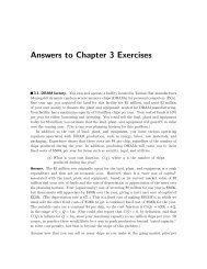
The situation of price competition with capacity constraints is illustrated in Figure 8.4.
D(p) is the demand curve. Two vertical lines represent each firm’s capacity. In this example,
Firm 2 is the one with greater capacity: k 2 > k 1 . The third vertical line, k 1 + k 2 , represents
total industry capacity.
f. For aficionados only: the above expression for firm i’s residual demand, D(p i) − k j, is only valid
under the assumption that the customers served by firm j are the ones with the greatest willingness
to pay. 5

Figure 8.4
Capacity constraints
p
... .... .... ... ... ... .... ... ... .... ....
P (k 1 + k 2 )
.. .. .. . . ... ... ... ... .. .. .. . . ... ... ... ... .. .. .. . . ... ... ... ... .. .. .. . .
r 2
d 2
D
q 1 , q 2
k 1 k 2 k 1 + k 2
Let P (Q) be the inverse demand curve, that is, the inverse of D(p). g Moreover, let
P (k 1 + k 2 ) be the price level such that, if both firms were to set p = P (k 1 + k 2 ), total
demand would be exactly equal to total capacity. This price level is simply derived from
the intersection of the demand curve with the total capacity curve. We will now argue that
the equilibrium of the price-setting game consists of both firms setting p i = P (k 1 + k 2 ). In
other words, firms set prices such that total demand equals industry capacity.
Let us consider Firm 2’s optimization problem assuming that Firm 1 sets p 1 = P (k 1 +k 2 ).
Can Firm 2 do better than setting p 2 = p 1 = P (k 1 + k 2 )? One alternative strategy is to
set p 2 < P (k 1 + k 2 ). By undercutting its rival, Firm 2 receives all of the market demand.
However, since Firm 2 is already capacity constrained when it sets p 2 = P (k 1 + k 2 ), setting
a lower price does not help: on the contrary, Firm 2 receives lower profits by setting a lower
price (same output sold at a lower price).
What about setting a price higher than P (k 1 + k 2 )? The idea is that, since Firm 1 is
capacity constrained when p 1 = P (k 1 + k 2 ), Firm 2 will receive positive demand even if it
prices above Firm 1. Figure 8.4 depicts Firm 2’s residual demand, d 2 , under the assumption
that p 2 > p 1 and p 1 = P (k 1 + k 2 ): Firm 2 gets D(p 2 ) minus Firm 1’s output, k 1 , so d 2 is
parallel to D, the difference being k 1 . The figure also depicts Firm 2’s marginal revenue
curve, r 2 . As can be seen, marginal revenue is greater than marginal cost (zero) for every
value of output less than Firm 2’s capacity. This implies that setting a higher price than
P (k 1 + k 2 ), which is the same as selling a lower output than q 2 = k 2 , would imply a lower
profit: the revenue loss (the positive marginal revenue) is greater than the cost saving (the
value of marginal cost, which is zero).
A similar argument would hold for Firm 1 as well: given that p 2 = P (k 1 + k 2 ), Firm 1’s
optimal strategy is to set p 1 = P (k 1 + k 2 ). We thus conclude that p 1 = p 2 = P (k 1 + k 2 )
is indeed an equilibrium. Notice that, if capacity levels were very high, then the above
argument would not hold; that is, it might be optimal for a firm to undercut its rival’s
g. D(p), the direct demand curve (or simply demand curve), corresponds to taking price as the independent
variable, that is, quantity as a function of price; P (Q), the inverse demand curve, corresponds
to taking quantity as the independent variable, that is, price as a function of quantity.

Box 8.2. WorldCom and the U.S. telecoms price wars. 7
After merging with MCI in 1998, WorldCom became one of the leading players in the
global telecom industry. Central to WorldCom’s strategy was tapping into the Internet’s
rapid growth by expanding fiber optic capacity. The company’s mantra — shared
by many industry analysts — was that Internet traffic was doubling every 100 days.
Unfortunately, WorlCom was not the only game in town: “In 1998 anyone who announced
plans to layer fiber could get $1 billion from Wall Street, no questions asked.”
And many did. Moreover, the estimates of the growth in Internet traffic turned out
to be wildly exaggerated: what happened in the early 1990s was no longer true by the
late 1990s.
As a result, the telecom industry imploded. Excess capacity fueled vicious price wars.
Many startups filed for bankruptcy, dumping their capacity on the market at bargainbasement
prices. Meanwhile, the long-reliable long-distance voice market lost share to
wireless. WorldCom wasn’t immune to these events, and its stock price fell by 70%
during 2000.
One analyst summarized the events as follow: “WorldCom’s main transgression was to
pour gasoline on the Internet fire. The technological revolution was pretty powerful as
it was, but WorldCom made it much worse than it would have been.”
price. However, if capacities are relatively small, then the result obtains that equilibrium
prices are such that total demand equals total capacity. 6 In summary:
If total industry capacity is low in relation to market demand, then equilibrium prices
are greater than marginal cost.
Conversely, if industry capacity is very high, then an equilibrium with positive margins
may turn into the Bertrand trap we saw earlier. Box 8.2 summarizes the case of WorlCom
and the long-distance telecommunications industry: a glut of fiber optic capacity pushed
prices down to marginal cost, leading many firms to bankruptcy and sowing the seeds of
WorldCom’s eventual demise.
8.2. The Cournot model
In the previous section, we concluded that, if firms’ sales are limited by the capacity they
created beforehand, then in equilibrium firms set prices such that total demand just clears
total capacity. The same applies for the choice of output level, to the extent that firms must
first produce a certain amount and then set prices to sell the output previously produced.
This analysis can be taken one step back: what output levels should firms choose in the first
place? Suppose that output decisions are made simultaneously before prices are chosen.
Based on the above analysis, firms know that, for each pair of output choices (q 1 , q 2 ),
equilibrium prices will be p 1 = p 2 = P (q 1 + q 2 ). This implies that firm i’s profit is given by

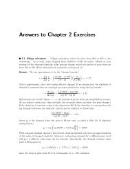
Figure 8.5
Firm 1’s optimum
p
P (q 2 )
D
c
P (q ′ 1 + q 2 )
r 1 (q 2 )
.
.
.
.
.
.
.
.................................................................................................................................................... ....................................................................................................................................................
.
.
.
.
.
.
.
q 2
d 1 (q 2 )
MC
q 1 , q 2
q ∗ 1(q C ) q ∗ 1(q 2 ) q ∗ 1(0) q ′ 1 q ′ 1 + q 2
(
π i = q i P (q1 + q 2 ) − c ) , assuming, as before, constant marginal cost.
The game where firms simultaneously choose output levels is known as the Cournot
model. 8 Specifically, suppose there are two firms in a market for a homogeneous product.
Firms choose simultaneously the quantity they want to produce. The market price is then
set at the level such that demand equals the total quantity produced by both firms.
As in Section 8.1, our goal is to derive the equilibrium of the model, that is, the equilibrium
of the game played between the two firms. Also as in Section 8.1, we do so in two
steps. First, we derive each firm’s optimal choice given its conjecture of what the rival does,
that is, the firm’s best response. Second, we put the best response mappings together and
find a mutually consistent combination of actions and conjectures.
Suppose that Firm 1 believes Firm 2 is producing quantity q 2 . What is Firm 1’s optimal
quantity? The answer is provided by Figure 8.5. If Firm 1 decides not to produce anything,
then price is given by P (0 + q 2 ) = P (q 2 ). If Firm 1 instead produces q 1 ′ , then price is given
by P (q 1 ′ + q 2). More generally, for each quantity that Firm 1 might decide to set, price is
given by the curve d 1 (q 2 ), which is referred to as Firm 1’s residual demand: it gives all
possible combinations of Firm 1’s quantity and price for a given a value of q 2 .
Having derived Firm 1’s residual demand, the task of finding Firm 1’s optimum is now
similar to finding the optimum under monopoly, which we have already done in Chapter
5. Basically, we must determine the point where marginal revenue equals marginal cost.
Marginal cost is constant by assumption and equal to c. Marginal revenue is a curve with
twice the slope of d 1 (q 2 ) and with the same vertical intercept. h The point at which the two
curves intersect corresponds to quantity q1 ∗(q 2), Firm 1’s best response to Firm 2’s strategy.
Notice that Firm 1’s optimum, q1 ∗(q 2), depends on its belief of what Firm 2 chooses.
In order to find an equilibrium, we are interested in deriving Firm 1’s optimum for other
possible values of q 2 . Figure 8.5 considers two other possible values of q 2 . If q 2 = 0,
then Firm 1’s residual demand is effectively the market demand: d 1 (0) ≡ D. The optimal
h. This results from our assumption that demand is linear. In general, the marginal revenue curve has
the same intercept as the demand curve and a higher slope (in absolute value), not necessarily twice
the slope of the demand curve.

solution, not surprisingly, is for Firm 1 to chose the monopoly quantity: q1 ∗(0) = qM , where
q M is the monopoly quantity. If Firm 2 were to chose the quantity corresponding to perfect
competition, that is q 2 = q C , where q C is such that P (q C ) = c, then Firm 1’s optimum
would be to produce zero: q1 ∗(qC ) = 0. In fact, this is the point at which marginal cost
intercepts the marginal revenue corresponding to d 1 (q C ).
It can be shown that, given a linear demand and constant marginal cost, the function
q1 ∗(q 2) — Firm 1’s best response mapping — is also linear. Since we have two points, we
can draw the entire function q1 ∗(q 2). This is done in Figure 8.6. Notice that the axes are
now different from the previous figures. On the horizontal axis, we continue measuring
quantities, specifically, Firm 2’s quantity, q 2 . On the vertical axis, we now measure Firm
1’s quantity, q 1 , not price.
Algebraic derivation. Throughout this chapter, in parallel with the graphical derivation
of equilibria, I also present the correponding algebraic derivation. Except for some results
in the next section, algebra is not necessary for the derivation of the main results; but it
may help, especially if you are familiar with basic algebra and calculus. Let me start with
the algebraic derivation of Firm 1’s best response. Suppose that (inverse) demand is given
by P (Q) = a − b Q, whereas cost is given by C(q) = c q, where q is the firm’s output and
Q = q 1 + q 2 is total output.
Firm 1’s profit is
π 1 = P q 1 − C(q 1 ) = ( a − b (q 1 + q 2 ) ) q 1 − c q 1
The first-order condition for the maximization of π 1 with respect to q 1 , ∂ π 1 /∂ q 1 = 0, is
or simply
−b q 1 + a − b (q 1 + q 2 ) − c = 0
q 1 = a − c − q 2
2 b 2
Since this gives the optimum q 1 for each value of q 2 , we have just derived the Firm 1’s
best response, q1(q ∗ 2 ):
q ∗ 1(q 2 ) = a − c
2 b
− q 2
2
(1)
We are now ready for the last step in our analysis, that of finding the equilibrium. An
equilibrium is a point at which firms choose optimal quantities given what they conjecture
the other firm does; and those conjectures are correct. Specifically, an equilibrium will
correspond to a pair of values (q 1 , q 2 ) such that q 1 is Firm 1’s optimal response given q 2
and, conversely, q 2 is Firm 2’s optimal response given q 1 .
We have not derived Firm 2’s best response. However, given our assumption that both
firms have the same cost function, we conclude that Firm 2’s best response, q2 ∗(q 1), is the
symmetric of Firm 1’s. We can thus proceed to plot the two best responses in the same
graph, as in Figure 8.6.
As in the case of the Bertrand model (see Section 8.8.1), the equilibrium point in the
Cournot model is then given by the intersection of the best response mappings, point N. In

Figure 8.6
Cournot model: best responses and equilibrium.
q 1
q 2
q ∗ 2 (q 1)
. .
q M
̂q
M
N
•
C
. .
q ∗ 1 (q 2)
q C . .. ... ... ... ... .... ... .... .. ... ... ... .... .. ... ... .............
̂q q M q C
fact this is the point at which q 1 = q ∗ 1 (q 2) (because the point is on Firm 1’s best response)
and q 2 = q ∗ 2 (q 1) (because the point is on Firm 2’s best response). i
Algebraic derivation (cont). We now proceed with our algebraic derivation. In equilibrium,
it must be that Firm 1 chooses an output that is optimal given what it expects Firm
2’s output to be. If Firm 1 expects Firm 2 to produce q e 2, then it must be ̂q 1 = q ∗ 1(q e 2).
Moreover, in equilibrium Firm 1’s conjecture regarding Firm 2’s choice should be correct:
q e 2 = ̂q 2 . Together, these conditions imply that ̂q 1 = q ∗ 1(̂q 2 ). The same conditions apply for
Firm 2, that is, in equilibrium it must also be the case that ̂q 2 = q ∗ 2(̂q 1 ). An equilibrium
is thus defined by the system of equations
̂q 1 = q ∗ 1(̂q 2 )
̂q 2 = q ∗ 2(̂q 1 )
Equation (1) gives Firm 1’s best response. We can thus write the first equation of the
above system as
̂q 1 = a − c − ̂q 2
2 b 2
Since the two firms are identical (same cost function), the equilibrium will also be symmetric,
that is, ̂q 1 = ̂q 2 = ̂q. j We thus have
Solving for ̂q, this yields
̂q = a − c
2 b
̂q = a − c
3 b
− ̂q 2
i. The equilibrium concept we are using here is that of Nash equilibrium, or Nash-Cournot equilibrium,
thus the notation N. In general, more than one equilibrium can exist. However, when the demand
curve is linear and marginal cost is constant there exists one equilibrium only.
j. For aficionados: in general, the fact that a game is symmetric does not imply that its equilibrium is
symmetric as well. However, when best responses are linear as in the present case symmetry of the
model implies symmetry (and uniqueness) of the equilibrium.

Monopoly, duopoly, and perfect competition. Duopoly is an intermediate market
structure, between monopoly (maximum concentration of market shares) and perfect competition
(minimum concentration of market shares). One would expect equilibrium price
and output under duopoly also to lie between the extremes of monopoly and perfect competition.
This fact can be checked based on Figure 8.6. Recall that each firm’s best response
intercepts the axes at the values q M and q C . Therefore, a line with slope −1 intersecting
the axes at the farther extremes of the best response mappings unites all points such that
̂q 1 +̂q 2 = q C (line C in Figure 8.6). Likewise, a line with slope −1 intersecting the axes at the
closer extremes of the best response mappings unites all points such that ̂q 1 + ̂q 2 = q M (line
M in Figure 8.6). We can see that the Cournot equilibrium point, N, lies between these
two lines. This implies that total output under Cournot is greater than under monopoly
and lower than under perfect competition.
To summarize,
Under output competition (Cournot), equilibrium output is greater than monopoly
output and lower than perfect competition output. Likewise, duopoly price is lower
than monopoly price and greater than price under perfect competition.
See Exercise 8.14 for the analytical version of this idea. In Chapter 10, I present a more
general result: in an oligopoly with n firms, equilibrium price is closer to perfect competition
the greater n is.
A “dynamic” interpretation of the Cournot equilibrium. It is easy to understand why
the Cournot equilibrium is a stable solution: no firm would have an incentive to choose
a different output. In other words, each firm is choosing an optimal strategy given the
strategy chosen by its rival. But: is the Cournot equilibrium a realistic prediction of what
will happen in reality?
The equilibrium concept we have used is that of Nash equilibrium, first introduced in
Chapter 7. There I presented a variety of possible justifications for the concept of Nash
equilibrium. Here I present an argument, first proposed by Cournot himself, which is similar
to the idea of solution by elimination of dominated strategies.
Although the Cournot model is a static game, let us consider the following dynamic
interpretation. At time t = 1, Firm 1 chooses some output level. Then, at time t = 2, Firm
2 chooses the optimal output level given Firm 1’s output choice. At time t = 3, it’s again
Firm 1’s turn to choose an optimal output given Firm 2’s current output; and so on: Firm
1 chooses output at odd time periods, and Firm 2 at even time periods.
Figure 8.7 gives an idea of what this dynamic process might look like. We start from
a point in the horizontal axis (q2 ◦ , Firm 2’s output at time zero). At time t = 1, we move
vertically towards Firm 1’s best response (Firm 1 is optimizing). At time t = 2, we move
horizontally to Firm 2’s best response (Firm 2 is optimizing). At time t = 3, we move
again vertically toward Firm 1’s best response. And so on. As can be seen from the figure,
the dynamic process converges to the Cournot equilibrium. In fact, no matter what the
initial situation, we always converge to the Nash equilibrium. This is reassuring, insofar as
it provides an additional motivation for the idea of Cournot equilibrium.

Figure 8.7
Convergence to Cournot equilibrium
q 1
q 2
q ∗ 2(q 1 )
............
.
.................................................
.
.
q ∗ 1(q 2 )
...........
..................................................................................................
.
.
q ◦ 2
8.3. Bertrand vs. Cournot
The two models of duopoly competition presented in the previous sections, though similar
in assumptions, are in stark contrast when it comes to predicted behavior. The Cournot
model predicts that price under duopoly is lower than monopoly price but greater than under
perfect competition. The Bertrand model, by contrast, predicts that duopoly competition
is sufficient to drive prices down to marginal cost level, that is, two firms are sufficient to
bring price down to the price level under perfect competition.
This contrast suggests two questions: Which model is more realistic? Why should we
consider more than one model instead of just choosing the “best” one? The answer to both
questions is that industries differ; and some industries are more realistically described by the
Cournot model, whereas other industries are more realistically described by the Bertrand
model.
Specifically, suppose that firms must make capacity (or output) decision in addition to
pricing decisions. In this context, the crucial aspect that selects Cournot or Bertrand as
the right model is the relative timing of each decision (output and pricing). As I showed in
Chapter 7, games with two strategic decisions are best modeled as two-stage games, with
the long-run decisions taken in the first stage and the short-run decisions taken in the second
one. The idea is that the short-run decisions (second stage) are taken given the values of
the long-run decisions (first stage).
Suppose that capacity or output is a long-run decision with respect to prices. In other
words, suppose that it is easier to adjust price than it is to adjust capacity or output. Then,
the “right” model is one where firms first set capacity and output and then prices. From
the analysis of the previous sections, we know this corresponds to the Cournot model.
By contrast, suppose that output is a short-run decision with respect to prices, that is,
it is easier to adjust output levels that it is to adjust prices. Then, the “right” model is
one where firms first set prices and then output levels. Although we have not presented
the Bertrand model as such, this is essentially what it corresponds to. In the Bertrand
model, firms simultaneously set prices and receive demand based on those prices. Implicitly
assumed in the model is that firms produce an output exactly equal to the quantity

demanded, that is, output is perfectly adjusted to the quantity demanded at the prices
(initially) set by firms.
To summarize:
If capacity and output can be adjusted easily, then the Bertrand model describes
duopoly competition better. If output and capacity are difficult to adjust, then the
Cournot model describes duopoly competition better.
Most real-world industries seem closer to the case when capacity is difficult to adjust. In
other words, capacity or output decisions are normally the long-run variable, prices being
set in the short run. Examples include wheat, cement, steel, cars, computers. Consider,
for instance, the market for video-game consoles. On August 1999, Sony cut the price of
its system from $129 to $99. One hour after Sony’s price-change press release, Nintendo
published its own release announcing a price cut to match Sony’s. 9 Aggressive pricing by
Sony and Nintendo boosted demand for their products. In fact, Nintendo suffered severe
shortages during the 1999 holiday season. These events suggest that, in the context of
video-game systems, prices are easier to adjust than quantities. The Cournot model would
then seem a better approximation to the behavior of the industry.
There are, however, situations where capacities — or at least output levels — are adjusted
more rapidly than prices. Examples include software, insurance and banking. A
software company, for example, can easily produce additional copies of its software almost
on demand; sometimes, in fact, it will simply ship a copy electronically. In this sense, the
Bertrand model would provide a better approximation than the Cournot model. k
8.4. The models at work: comparative statics
What is the use of solving models and deriving equilibria? Models are simplified descriptions
of reality, a way of understanding a particular situation. Once we understand how a given
market works, we can use the model to predict how the market will change as a function
of changes in various exogenous conditions, e.g., the price of an input or of a substitute
product. This exercise is known in economics as comparative statics: the meaning of the
expression is that we compare two equilibria, with two sets of exogenous conditions, and
predict how a shift in one variable will influence the other variables. The word “statics”
implies that we are not predicting the dynamic path that takes us from one equilibrium to
the other, but rather answering the question “once all of the adjustments have taken place
and we are back in equilibrium, what will things look like.”
In this section, I look at some examples of how the Cournot and Bertrand models can
be used to perform comparative statics. Some of the practice and challenge exercises at the
end of the chapter, especially Exercise 8.17, take the idea of comparative statics a few steps
further.
Input costs and output price. Suppose the market for transatlantic flights between
London and New York is served by two firms, American Airlines (AA) and British Airways
k. There are, however, other aspects to be taken into account in an industry like software: product
differentiation (cf Chapter 15) and network effects (cf Chapter 18).

Figure 8.8
Optimal solution after increase in marginal cost
p
c ′ = 1.4 c
c
.
.
.
.
.
.
.
.
.
.
.
.
.
.
.
.
.
.
.
.
.
.
.
.
.
.
.
.
.
.
.
.
.
.
.
.
.
.
.
.
.
.
.
.
.
.
.
.
.
.
.
.
q
q M ′
q M q C ′
q C
(BA). Both firms have the same marginal cost, which can be divided into labor costs (50%)
and fuel (50%), and is initially at $300. Suppose fuel costs go up by 80%. What will happen
to transatlantic airfares between London and New York?
Suppose AA and BA compete à la Cournot. This assumption might be justified, in line
with the discussion in the previous section, by the fact that firms must decide beforehand
how much capacity (aircraft) to allocate to the market.
Looking back at the graphical derivation of the Cournot equilibrium (page 10), we see
that each firm’s best response depends on its marginal cost. l We should thus compute a
new best response based on the higher value of marginal cost. In Figure 8.8, we compute
the new q1 ∗(0) (that is, qM ′ ), and the new value q C ′ such that q1 ∗(qC ′ ) = 0, the two extreme
points of the best response. Based on these extreme points, we can draw the new best
response. This is done in Figure 8.9. Notice how, under Cournot competition, an increase
in marginal cost implies a downward shift of the best response. This is an important fact
which will reappear in different applications.
By symmetry, we know that both firms will experience the same shift in their best response.
We thus have everything that is needed in order to determine the new equilibrium,
which is depicted in Figure 8.9. The new equilibrium point is denoted by N ′ . For comparison,
the previous equilibrium, N, is also shown. As expected, each firm’s output as well as
total output are lower in the new equilibrium; it follows that price is higher.
Algebraic derivation. Let us now solve the problem algebraically. As we saw in Section
8.2, the equilibrium output in a (symmetric) Cournot equilibrium is given by
̂q = a − c
3 b
l. Firm 1’s best response depends on the rival’s output but not on the rival’s marginal cost. In equilibrium,
the rival’s output will depend on its marginal cost, so that, indirectly, Firm 1’s output will
depend on Firm 2’s marginal cost. However, when we talk about the best response, what is important
is whether Firm 1’s output depends directly on Firm 2’s marginal cost, which is not the case.

Figure 8.9
Cournot equilibrium after increase in marginal cost (N ′ )
45 ◦
. .
N ′ q ∗ 2(q 1 )
• •N
q ∗ 1(q 2 )
̂q 1
̂q 2 q M ′
q M q C ′
q C
q 1
.... .... .... .... .... ... .... ... ... ... ... .... .... .
.......
q 2
. .
Total output is therefore
̂Q = 2 a − c
3 b
Substituting in the demand function, we obtain equilibrium price:
We thus have
̂p = a − b ̂Q
= a − b 2 a − c
3 b
= a + 2 c
3
d ̂p
dc = 2 3
In economics jargon, we say that the pass through rate is 2 3
≈ 66%. To put a dollar value
on the price change, note that an 80% increase in fuel costs implies a 80%×50%=40%
increase in marginal cost, or a 40% × 300 = $120 increase. This increase in marginal cost
is experienced by both firms. It follows that price increases by 2 3
120 = $80.
(2)
Exchange rate fluctuations and market shares. Consider a duopoly with two different
firms from two different countries. For example, two producers of microchips, one in Japan
(Firm 1) and one in the U.S. (Firm 2). The market for microchips is in US$ (that is, all
sales are made in US$). However, the costs of the Japanese firm are paid in Japanese Yen.
(The American firm’s costs are in US$.)
Suppose that firms compete à la Cournot. In fact, this is one case where the reducedform
interpretation of the Cournot model seems appropriate: firms set production capacities
and then set prices (given capacities), the result of the two-stage game being identical to
Cournot competition.
In an initial equilibrium, both firms have the same cost and the market is divided equally
between the two. Moreover, equilibrium price is p = $24. One question which comparative

Figure 8.10
Cournot equilibrium after exchange rate devaluation
q 1
45 ◦
q 2
q ∗ 2(q 1 )
̂q 1
̂q 2
• N ′
N
•
q ∗ 1(q 2 )
... .... .... .... .... ... ... ... .... .
............
. .
statics might help to answer is: What is the impact on market shares of a 50% devaluation
of the Yen?
Since the market is in $US, a shift in the exchange rate will change the Japanese firm’s
marginal cost in dollars, while keeping the U.S. firm’s marginal cost constant. Specifically,
suppose that both firms start with marginal cost c. Then the Japanese firms marginal cost
will change to c/e as a result of the devaluation, where e is the exchange rate in Yen/$.
For example, suppose marginal cost was initially $12 for the U.S. firm and Y1200 for
the Japanese firm; and that the initial exchange rate was 100 Y/$. This implies that the
Japanese firm’s marginal cost in US$ was 1200/100 = $12. A 50% devaluation of the
Yen means that $1 is now worth Y150. The Japanese firm’s marginal cost in US$ is now
1200/150 = $8. We thus have to compute the new equilibrium where one of the firm’s
marginal cost is lower.
In the previous application, we saw that an increase in marginal cost implies a downward
shift in the best response. By analogy, we now deduce that the Japanese firm’s best response
will shift upwards as a result of the reduction in its marginal cost (in US$). Since only the
Japanese firm’s best response has changed, we are now ready to determine the equilibrium
shifts resulting from a Yen devaluation. This is done in Figure 8.10, where the Japanese
firm’s output is measured in the vertical axis and the American firm’s on the horizontal
one. As can be seen, the new equilibrium point N ′ is above the 45 ◦ line, that is, the
Japanese firm’s output is now greater than the American firm’s. This is not surprising, as
the Japanese firm has decreased its cost (in US$), whereas the U.S. firm’s cost remained
unchanged.
Algebraic computation. The graphical analysis has the limitation that it is difficult to
determine the precise value of market shares. The best strategy is then to solve the model
algebraically, which we do now. The first thing we must do is to determine the Cournot
equilibrium for the asymmetric case. From Section 8.2, we know that a firm’s best response
is given by
q1(q ∗ 2 ) = a − c − q 2
2 b 2

where c is marginal cost. Let Firms 1 and 2 marginal cost now be given by c 1 and c 2 ,
respectively. The two best response mappings are then given by
q ∗ 1(q 2 ) = a − c 1
2 b
q ∗ 2(q 1 ) = a − c 2
2 b
− q 2
2
− q 1
2
Substituting the first equation for q 1 in the second and imposing the equilibrium condition
q 2 = q2(q ∗ 1 ), we get
q 2 = a − c a−c 1
2 2 b
− q2 2
−
2 b 2
Solving for q 2 , we get
̂q 2 = a − 2 c 2 + c 1
3 b
Likewise,
̂q 1 = a − 2 c 1 + c 2
(3)
3 b
(The latter expression is obtained by symmetry; all we have to do is to interchange the
subscripts 1 and 2.) Total quantity is given by
̂Q = ̂q 1 + ̂q 2 = 2 a − c 1 − c 2
3 b
Finally, Firm 1’s market share. s 1 , is given by
(4)
s 1 = q 1
q 1 + q 2
= a − 2 c 1 + c 2
2 a − c 1 − c 2
(5)
It can be showed that s 1 > s 2 if and only if c 1 < c 2 . (Can you do it?) It follows that,
by decreasing its cost below its rival, the Japanese firm’s market share is greater than the
American’s.
Calibration. I would like to go beyond the expression on the right-hand side of (5) and put
an actual number to the value of s 1 . So far, all I know is that, initially, c 1 = c 2 , whereas,
after the devaluation, c 2 remains constant at $12, whereas c 1 drops to 12/1.5 = $8. As
can be seen from (5), in order to derive the numerical value of s 1 , I need to obtain the
value of a. The process of obtaining specific values for the model parameters based on
observable information about the equilibrium is know as model calibration.
Earlier, I determined that, in a symmetric Cournot duopoly,
p = a + 2 c
3
where c is the value of marginal cost. Solving with respect to a and plugging in the values
observed in the initial equilibrium, I get
a = 3 p − 2 c = 3 × 24 − 2 × 12 = 48
Given this value of a and given c 1 = 8 and c 2 = 12, I can now use (5) to compute the
Japanese firm’s market share:
s 1 =
48 − 2 × 8 + 12
2 × 48 − 8 − 12 ≈ 58%
In summary, a 50% devaluation of the Yen increases the Japanese firm’s market share to
58% from an initial 50%.

New technology and profits. Consider the industry for some chemical product, a
commodity that is supplied by two firms. Firm 1 uses an old technology and pays a marginal
cost of $15. Firm 2 uses a modern technology and pays a marginal cost of $12. In the current
equilibrium, price is at $20 per ton and output 13 million tons. How much would Firm 1
be willing to pay for the modern technology?
Quite simply, the amount that Firm 1 should be willing to pay for the technology is
the difference between its profits with lower marginal cost and its current profits. We
thus have to determine Firm 1’s equilibrium profits in two possible equilibria and compute
the difference. In a way, this problem is the reverse of the one examined before. In the
case of exchange-rate devaluation, we started from a symmetric duopoly and moved to an
asymmetric one. Now, we start from an asymmetric duopoly (Firm 2 has lower marginal
cost) and want to examine the shift to a symmetric duopoly, whereby Firm 1 achieves the
same marginal cost as its rival.
Algebraic derivation From (4), we know that total output is given by
Substituting in the demand function, we get
̂Q = ̂q 1 + ̂q 2 = 2 a − c 1 − c 2
3 b
̂p = a − b ̂Q = a + c 1 + c 2
3
(Notice that, in the particular case when c 1 = c 2 = c, we get (2), the equilibrium price in
the symmetric duopoly case.)
Given the expressions for Firm 1’s output (3) and for equilibrium price (6), we can
now compute Firm 1’s equilibrium profits:
π 1 = p q 1 − c 1 q 1
= a + c 1 + c 2
q 1 − c 1 q 1
(
3
)
a + c1 + c 2
=
− c 1 q 1
3
( ) a + c1 + c 2 a + c2 − 2 c 1
=
− c 1
3
3 b
= a + c 2 − 2 c 1
· a + c 2 − 2 c 1
3
3 b
( ) 2
a + c2 − 2 c 1
(6)
= 1 b
3
Finally, the value that Firm 1 would be willing to pay for the improved technology would
be the difference in the value of the above expression with c 1 = 15 and c 1 = 12. In order
to determine the precise value, we need, once again, to calibrate the model.
By analogy with the previous application, we can invert the price equation (6) to
obtain
a = 3 p − c 1 − c 2
Since p = 20, c 1 = 15, c 2 = 12, this implies that a = 3 × 20 − 15 − 12 = 33. Moreover, (4)
can be inverted to obtain
b = 2 a − c 1 − c 2
3 Q

Since Q = 13, it follows that b = (2 × 33 − 15 − 12)/(3 × 13) = 1. Therefore, in the initial
equilibrium, Firm 1’s profits are given by
( ) 2 33 + 12 − 2 × 15
̂π 1 =
=
3
( ) 2 15
= 25
3
whereas, with the new technology, profits would be given by
( ) 2 ( ) 2 33 + 12 − 2 × 12 21
̂π 1 =
= = 49
3
3
I conclude that Firm 1 should be willing to pay 49 − 25 = 24 for the new technology.
Given the units I worked with (price in $ per ton and quantity in million tons) this would
be $24 million.
Let us go back to where we started this section. Why is it useful to perform comparative
statics? Take for example the last application considered above. The question we posed
was: How much would Firm 1 (the inefficient firm) be willing to pay for an innovation
that reduces marginal cost to 12 (the efficient firm’s cost level)? Our analysis produced an
answer to this question: Firm 1 would gain 24 from adopting the more efficient technology.
Is it worth going through all the algebraic trouble to get this answer? A simpler estimate
for the gain might be the following: take Firm 1’s initial output as given and compute the
gain from reducing marginal cost. Since initial output is 5 (check), this calculation would
yield the number 5 × (15 − 12) = 15. This number greatly underestimates the true gain of
24. Why? The main reason is that, upon reducing marginal cost, Firm 1 becomes much
more competitive: not only does it increase its margin, it also increases its output.
Let us then consider an alternative simple calculation. Since Firm 1 will have a marginal
cost identical to Firm 2’s, we can estimate the gain by the difference between Firm 2’s and
Firm 1’s initial profits. Firm 2’s output (in the initial equilibrium) is 8 (check), whereas
price is given by 20; its profit is thus 8 × (20 − 12) = 64. Firm 1, in turn, is starting from
a profit of 5 × (20 − 15) = 25. We would thus estimate a gain of 64 − 25 = 39. This time
we are grossly overestimating the true value. Why? The main reason is that, when Firm
1 lowers marginal cost, duopoly competition heats up and price drops. As a result, Firm
2’s profit (which is now equal to Firm 1’s) also drops. In other words, the number π 2 − π 1
over-estimates the gain from technology adoption because it omits the effect of increased
competition.
The advantage of the equilibrium analysis — that is, comparative statics — is that it
takes into account all of the effects that follow from an exogenous change, such as a reduction
in one of the firm’s marginal cost. Taking the initial equilibrium values as constant may
lead to gross misestimation of the impact of an exogenous change, especially if the change
is significant in magnitude (as in the present example).
Exchange rates and sales margin. A French pharmaceutical firm is the sole domestic
producer of a given generic antidepressant. Its marginal cost is e2 per dose. Demand in
France is given by Q = 400−50 p (Q in millions of doses, p in e). There is a second producer
in India whose marginal cost is INR 150 (including transportation cost to the France). The
French regulatory system implies that firms must commit to prices for one year at a time.
Production capacity can be easily adjusted, since the firms produce several other medical

drugs. Suppose that the Indian rupee is devalued by 20% from its initial value of INR 50/e.
What impact does this have on the French firm’s profitability?
Given the nature of price and output decisions, the Bertrand model seems appropriate
for modeling the competition between the French and the Indian firm (Firms 1 and 2,
respectively). Initially, the Indian firm’s marginal cost in e is given by 150/50 = e3. Since
this is greater than the French firm’s marginal cost, we conclude that the French firm sets
a price p 1 = e3 (or perhaps a tad lower), which in turn implies a total profit of
π 1 = (400 − 50 × 3) × (3 − 2) = 250 (million e)
When the rupee devalues by 20%, the new exchange rate becomes 50 × (1 + 20%) = 60. It
follows that the Indian firm’s marginal cost expressed in e becomes 150/60= e 2.5. This
is still greater than e 2, so the French firm still corners the market. Its new profit level is
given by
π 1 = (400 − 50 × 2.5) × (2.5 − 2) = 137.5
which corresponds to a 45% drop in profits.
Summary
• Under price competition with homogeneous product and constant, symmetric marginal
cost (Bertrand competition), firms price at the level of marginal cost. • If total industry
capacity is low in relation to market demand, then equilibrium prices are greater than
marginal cost. • Under output competition (Cournot), equilibrium output is greater than
monopoly output and lower than perfect competition output. Likewise, duopoly price is
lower than monopoly price and greater than price under perfect competition. • If capacity
and output can be adjusted easily, then the Bertrand model describes duopoly competition
better. If output and capacity are difficult to adjust, then the Cournot model describes
duopoly competition better.
Key concepts
• oligopoly • duopoly • Bertrand trap • residual demand • comparative
statics • pass through rate • model calibration
Review and practice exercises
8.1. Bertrand in the real world. The Bertrand model of price competition suggests that,
under a given set of conditions, firms make zero economic profits even if there are only two
firms. However, there are many instances of industries with a small number of competitors
where firms appear to earn more than zero economic profits.

Give an example of an industry dominated by a couple of firms where profits are significant.
Explain why the predictions of the Bertrand model are not borne out.
8.2. Bertrand and zero profits. According to Bertrand’s theory, price competition
drives firms’ profits down to zero even if there are only two competitors in the market.
Why don’t we observe this in practice very often?
8.3. E-commerce. E-commerce represents an increasing fraction of economic transactions
in many different industries. Does e-commerce create a Bertrand trap? What is
special about e-commerce (and, more generally, the new economy) that makes the Bertrand
trap a dangerous trap? How can e-commerce firms avoid the trap?
8.4. Price discrimination. A monopolist is generally better off by price-discriminating.
What about a duopolist? Consider the special case when Market A is Firm 1’s “strong”
market, whereas market B is firm 2’s “strong” market.
8.5. Cournot model assumptions. Three criticisms are frequently raised against the
use of the Cournot oligopoly model: (i) firms normally choose prices, not quantities; (ii)
firms don’t normally take their decisions simultaneously; (iii) firms are frequently ignorant
of their rivals’ costs; in fact, they do not use the notion of Nash equilibrium when making
their strategic decisions. How would you respond to these criticisms? (Hint: in addition to
this chapter, you may want to refer to Chapter 7.)
8.6. Cournot vs. Bertrand. Which model (Cournot, Bertrand) would you think provides
a better approximation to each of the following industries: oil refining, internet access,
insurance. Why?
8.7. ByeByeCold. You are currently the sole seller of ByeByeCold, a revolutionary drug
that almost instantly eliminates cold symptoms. Although the production cost is only $.10
per dose, you sell ByeByeCold for $1.39 per dose, for a total profit of $900m a year. You
are currently considering licensing ByeByeCold to a second producer. Neither you nor your
competitor have any significant capacity constraints. One of your managers suggested, since
the firm would be sharing the market with a competitor, it would be appropriate to charge
a flat fee that covers half the current profits plus a generous margin; the value of $700m was
suggested. An alternative proposal would be to set a royalty fee of $.50 per dose. What is
your opinion?
8.8. French generics manufacturer. Consider the last problem in Section 8.4. Suppose
that a retailing campaign costing e 80m is expected to increase demand by 40%. Suppose
also that the current rupee/euro exchange rate is 50 INR/e. Should the French firm go
ahead with the campaign? One macroeconomics expert tells you that “it is likely that the
rupee will appreciate in the near future.” How would this influence your decision?
8.9. Karmania automobiles. There are two auto producers in Karmania, F1 and F2.

The cars they produce are essentially identical. The market inverse demand curve is given
by p = a − b Q, where p is price (in thousands of dollars); Q market output (in thousands
of units); and a and b are parameters. It is estimated that a = 25 and b = .1. Both F1 and
F2 have a marginal cost of 10 thousand dollars per car.
Competition in the Karmania auto market works as follows. At the beginning of each
year, both firms simultaneously and independently decide how many cars to produce. Then
the market price adjusts so that supply equals demand.
(a) Determine F1’s best response mapping.
(b) Determine the equilibrium of the game played between F1 and F2.
(c) Suppose that an increase in incomes shifts demand to p = 28 − 0.1 Q.
What do you expect will happen to price and the number of cars sold?
8.10. Ethanol. In the ethanol industry, each firm chooses what output to produce and
price is determined by aggregate output. Market demand is given by Q = 1500 − 2 p, where
Q is in million tons and p in $/ton. There are two producers and their marginal costs are
constant and given by c 1 = 340, c 2 = 420 (both in $/ton).
(a) Determine equilibrium price, output and market shares.
Firm 2 is currently considering two possible strategies: (a) a public opinion campaign that
would cost $1.15 billion and shift the demand curve to Q = 1520 − 2 p; (b) a capital
investment of $4.9 billion that would reduce marginal cost c 2 to 400 $/ton.
(b) Are investments (a) and (b) worthwhile in isolation? Are they worthwhile
if taken together? Justify your answer.
Challenging exercises
8.11. Cournot with n asymmetric firms. Consider an industry with n output setting
firms, each with constant marginal cost c i and fixed cost F i . Market demand is given by

p = a − b Q, where Q = ∑ n
i=1 q i.
(a) Show that firm i’s best-response mapping is given by qi ∗(Q −i) = a−c i
1
2 Q −i, where Q −i ≡ ∑ j≠i q j.
2 b −
(b) Show(
that, in equilibrium, total output is given by
̂Q = n a − ∑ )
n
i=1 c i / ( b (n + 1) ) . (Hint: add up all n first-order
conditions for profit maximization.)
(
(c) Show that equilibrium price is given by ̂p = a + ∑ )
n
i=1 c i /(n + 1)
(d) Show(
that, in equilibrium, firm i’s output level is given by
ˆq i = a − n c i + ∑ )
j≠i c j / ( b (n + 1) )
(e) Show that, in equilibrium, firm i’s profit is given by
(
ˆπ i = a − n c i + ∑ 2/
j≠i j) c (n + 1) 2 / b − F i
(f) Show that, in equilibrium, consumer surplus is given by
(
CS = 1
2 b
n a − ∑ ) 2
n
i=1 c i /(n + 1)
2
8.12. Elasticity rule (reprise). Show that the elasticity rule derived in Chapter 3, that
is (p − MC )/MC = −1/ɛ, holds under Cournot competition with linear demand and costs,
where MC is firm i’s marginal cost and ɛ its demand elasticity (not the market elasticity).
8.13. Efficiency loss under Cournot. Consider a market for a homogeneous product
with demand given by Q = 37.5 − P/4. There are two firms, each with constant marginal
cost equal to 30.
(a) Determine output and price under a Cournot equilibrium.
(b) Compute the efficiency loss as a percentage of the efficiency loss under
monopoly.
8.14. Equilibrium price under Cournot. Show analytically that equilibrium price under
Cournot is greater than price under perfect competition but lower than monopoly price.
8.15. Cournot with increasing marginal cost. Consider a duopoly for a homogenous
product with demand Q = 10−P/2. Each firm’s cost function is given by C = 10+q(q +1).
(a) Determine the values of the Cournot equilibrium.
(b) Re-compute the equilibrium values assuming that one of the firms —
say, firm 2 — has a cost function given by C = 10 + q(q + 1).
8.16. Cement. Two firms compete (a la Cournot) in the cement market. Demand for
cement is given by Q = 450 − 2 P . Firm 1’s marginal cost is constant at 50, firm 2’s at 40.

A technological innovation allows firms to reduce marginal cost by 6.
(a) How much would each firm be willing to pay for the innovation if it
were the only competitor to acquire it?
Suppose the innovation costs 600. Consider a “metagame” where firms first simultaneously
decide whether to acquire the innovation and then compete a la Cournot with whatever
marginal cost results form the first stage.
(b) What is the equilibrium of the 2 × 2 game played by firms at the
technology choice stage?
8.17. Cournot in the desktop computer industry. In 2010, global sales of Windows-based
desktop computers were 351 million units, whereas average price was $605. 10 The leading
market shares were as follows: HP, 17.9%; Acer, 13.9%; Dell, 12%; Lenovo, 10.9%; Asus,
5.4%; others, 39.3%. Suppose that the Cournot model provides a good approximation of
the industry’s behavior. Suppose moreover that inverse demand is given by p = a − b Q;
each firm has constant marginal cost; and that, from previous studies, the price elasticity
of market demand is estimated to be -0.5 (at the market equilibrium level).
(a) Based on the observable data, estimate each firm’s marginal cost and
margin.
(b) Suppose that Dell’s marginal cost decreases by 5%. Based on your
answer to the previous question, estimate the impact of this cost decrease
on equilibrium price and on Dell’s market share.

Endnotes
1. The Wall Street Journal, November 16, 1999.
2. The Bertrand model was first introduced by J. Bertrand, “Théorie Mathématique de la Richesse Sociale”,
Journal de Savants (1883), 499–508.
3. Sources: Shapiro, Carl, and Hal Varian (1999), Information Rules, Harvard Business School Press. Computer
Business Review, 16 November 1987. See http://www.cbronline.com/news/nynex puts phone book on cd (visited
October 2012). Walter R. Baranger, Taking In the Sites; Number, Please? 3 Routes to Phone Listings, The New
York Times, August 07, 1995.
4. This example is adapted from Shapiro, Carl, and Hal Varian (1998), Information Rules: A Strategic Guide to
the Network Economy, Cambridge, Mass.: Harvard Business School Press.
5. See Davidson, Carl, and Raymond Deneckere (1986), “Long-run Competition in Capacity, Short-run
Competition in Price, and the Cournot Model,” Rand Journal of Economics 17, 404-415; and Herk, Leonard F.
(1993), “Consumer Choice and Cournot Behavior in Capacity-constrained Duopoly Competition,” Rand Journal of
Economics 24, 399–417.
6. If capacity costs are sufficiently high, then firms’ capacity levels will surely be sufficiently low that the above
result holds. However, it can be shown that, even if capacity costs were low, the same would be true. See Kreps,
David M. and José A. Sheinkman (1983), “Capacity Precommitment and Bertrand Competition Yield Cournot
Outcomes,” Bell Journal of Economics 14, 326–337.
7. Sources: Andy Kessler, “Bernie Bites the Dust,” The Wall Street Journal, May 1, 2002. Ken Belson,
“WorldCom’s Audacious Failure and Its Toll on an Industry,” The New York Times, January 18, 2005.
8. Cournot, Agustin, Recherches sur les Principes Mathématiques de la Théorie des Richesses (1838). English
translation edited by N. Bacon, New York: Macmillan, 1897.
9. Source: The Wall Street Journal, August 17, 1999.
10. Sources: http://en.wikipedia.org/wiki/Market share of personal computer vendors,
http://www.statista.com/statistics/203759/average-selling-price-of-desktop-pcs-worldwide/