8 Oligopoly - Luiscabral.net

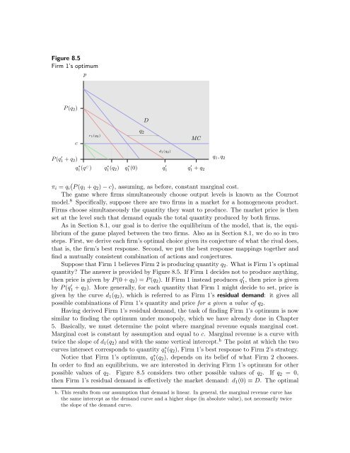
Figure 8.5
Firm 1’s optimum
p
P (q 2 )
D
c
P (q ′ 1 + q 2 )
r 1 (q 2 )
.
.
.
.
.
.
.
.................................................................................................................................................... ....................................................................................................................................................
.
.
.
.
.
.
.
q 2
d 1 (q 2 )
MC
q 1 , q 2
q ∗ 1(q C ) q ∗ 1(q 2 ) q ∗ 1(0) q ′ 1 q ′ 1 + q 2
(
π i = q i P (q1 + q 2 ) − c ) , assuming, as before, constant marginal cost.
The game where firms simultaneously choose output levels is known as the Cournot
model. 8 Specifically, suppose there are two firms in a market for a homogeneous product.
Firms choose simultaneously the quantity they want to produce. The market price is then
set at the level such that demand equals the total quantity produced by both firms.
As in Section 8.1, our goal is to derive the equilibrium of the model, that is, the equilibrium
of the game played between the two firms. Also as in Section 8.1, we do so in two
steps. First, we derive each firm’s optimal choice given its conjecture of what the rival does,
that is, the firm’s best response. Second, we put the best response mappings together and
find a mutually consistent combination of actions and conjectures.
Suppose that Firm 1 believes Firm 2 is producing quantity q 2 . What is Firm 1’s optimal
quantity? The answer is provided by Figure 8.5. If Firm 1 decides not to produce anything,
then price is given by P (0 + q 2 ) = P (q 2 ). If Firm 1 instead produces q 1 ′ , then price is given
by P (q 1 ′ + q 2). More generally, for each quantity that Firm 1 might decide to set, price is
given by the curve d 1 (q 2 ), which is referred to as Firm 1’s residual demand: it gives all
possible combinations of Firm 1’s quantity and price for a given a value of q 2 .
Having derived Firm 1’s residual demand, the task of finding Firm 1’s optimum is now
similar to finding the optimum under monopoly, which we have already done in Chapter
5. Basically, we must determine the point where marginal revenue equals marginal cost.
Marginal cost is constant by assumption and equal to c. Marginal revenue is a curve with
twice the slope of d 1 (q 2 ) and with the same vertical intercept. h The point at which the two
curves intersect corresponds to quantity q1 ∗(q 2), Firm 1’s best response to Firm 2’s strategy.
Notice that Firm 1’s optimum, q1 ∗(q 2), depends on its belief of what Firm 2 chooses.
In order to find an equilibrium, we are interested in deriving Firm 1’s optimum for other
possible values of q 2 . Figure 8.5 considers two other possible values of q 2 . If q 2 = 0,
then Firm 1’s residual demand is effectively the market demand: d 1 (0) ≡ D. The optimal
h. This results from our assumption that demand is linear. In general, the marginal revenue curve has
the same intercept as the demand curve and a higher slope (in absolute value), not necessarily twice
the slope of the demand curve.