8 Oligopoly - Luiscabral.net

More documents

Recommendations

Info

market demand. Take, for example, the cola market. In the U.S. and in many other countries, Pepsi and Coke are the two main competitors. Brand allegiance tends to be very high and cross-price elasticity tends to be relatively close to zero. By lowering its price, Coke may increase its sales a bit, but it will certainly not capture all of the market demand (as assumed under Bertrand competition). The issues of product differentiation and brand allegiance are examined in Chapters 15 and 16. 2. Dynamic competition. The Bertrand model assumes that firms compete in one period only; that is, price is chosen once and for all. One of the likely consequences of undercutting a rival’s price is that the latter will retaliate by lowering its price too, possibly initiating a price war. For example, if the BP gas station lowers its price today, it may attract additional customers who were previously filling up at the Exxon gas station across the street; but before long the Exxon gas station is bound to respond. In that case, undercutting does not guarantee a firm total market demand, except perhaps in the very short run. The possibility of retaliation is not considered in the Bertrand model because of its static nature. In the next chapter, I will consider dynamic games and show that, even when firms set prices and the product is homogeneous, there exist equilibria where price is strictly greater than marginal cost. 3. Asymmetric costs. One important assumption in the simple version of the Bertrand model I considered above is that both firms have the same marginal cost. As we will see below, if one of the firms has a lower marginal cost (a “cost leader”) then it is no longer true that both firms earn zero profits. 4. Capacity constraints. By undercutting the rival, a Bertrand duopolist receives all of the market demand. But what good is this if the firm does not have sufficient capacity to satisfy all of this demand? In other words, one important assumption of the Bertrand model is that firms have no capacity constraints. Below I show that, if there are capacity constraints, then the nature of competition may change considerably. Price competition with different costs. Consider the Portuguese wholesale gasoline market. There are essentially two sellers (that is, two supply sources): Galp, which owns all of the country’s refineries; and imports. Typically, the import price is greater than Galp’s cost. As a result, Galp supplies all retailers at the import price and effectively maintains a 100% market share in wholesale gasoline sales (that is, imports represent a very small share of total sales). In sum, although the product is relatively homogeneous and competition is based on price, Galp sells at a positive margin, the reason being that Galp has a lower marginal cost than its competitors. The simple version of the Bertrand model I considered before assumed that both firms had the same marginal cost. Suppose now that one of the firms, say Firm 1, has a lower marginal cost than its rival. The situation is depicted in Figure 8.3. The best response curves are derived as before: firm i undercuts the rival all the way down to its marginal cost — that is, all the way down to firm i’s marginal cost. In this case, since Firm 1 has a lower marginal cost, its best response mapping extents to lower values than Firm 2’s. As a result, the point where the two best responses cross — the Nash equilibrium of the game
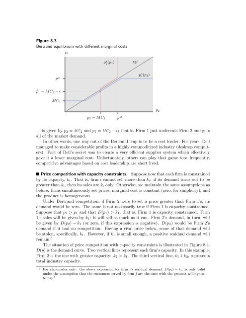
Figure 8.3 Bertrand equilibrium with different marginal costs p ∗ 2(p 1 ) 45 ◦ p ∗ 1(p 2 ) p M p 2 = MC 2 p M p 1 ... .... .... .... .... .... .... .... .... .... .... .... .... .... .... .... ... .... .... .... .... .... .... .... .... .... .... .... .... .... .... .... .... . .................... p 2 ̂p 1 = MC 2 − ɛ • ... ..... .... .... .... .... .... .. . .... ... .... .... .... .... ..... .... ... .... .... .... .... .... . ............ MC 1 — is given by p 2 = MC 2 and p 1 = MC 2 − ɛ; that is, Firm 1 just undercuts Firm 2 and gets all of the market demand. In other words, one way out of the Bertrand trap is to be a cost leader. For years, Dell managed to make considerable profits in a highly commoditized industry (desktop computers). Part of Dell’s secret was to create a very efficient supplier system which effectively gave it a lower marginal cost. Unfortunately, others can play that game too: frequently, competitive advantages based on cost leadership are short lived. Price competition with capacity constraints. Suppose now that each firm is constrained by its capacity, k i . That is, firm i cannot sell more than k i : if its demand turns out to be greater than k i , then its sales are k i only. Otherwise, we maintain the same assumptions as before: firms simultaneously set prices, marginal cost is constant (zero, for simplicity), and the product is homogeneous. Under Bertrand competition, if Firm 2 were to set a price greater than Firm 1’s, its demand would be zero. The same is not necessarily true if Firm 1 is capacity constrained. Suppose that p 2 > p 1 and that D(p 1 ) > k 1 , that is, Firm 1 is capacity constrained. Firm 1’s sales will be given by k 1 : it will sell as much as it can. Firm 2’s demand, in turn, will be given by D(p 2 ) − k 1 (or zero, if this expression is negative). D(p 2 ) would be Firm 2’s demand if it had no competition. Having a rival price below, some of that demand will be stolen, specifically, k 1 . However, if k 1 is small enough, a positive residual demand will remain. f The situation of price competition with capacity constraints is illustrated in Figure 8.4. D(p) is the demand curve. Two vertical lines represent each firm’s capacity. In this example, Firm 2 is the one with greater capacity: k 2 > k 1 . The third vertical line, k 1 + k 2 , represents total industry capacity. f. For aficionados only: the above expression for firm i’s residual demand, D(p i) − k j, is only valid under the assumption that the customers served by firm j are the ones with the greatest willingness to pay. 5
Page 1 and 2: 8 Oligopoly So far, we have looked
Page 3 and 4: Figure 8.1 Bertrand game with limit
Page 5: Box 8.1. Digital yellow pages: from
Page 9 and 10: Box 8.2. WorldCom and the U.S. tele
Page 11 and 12: solution, not surprisingly, is for
Page 13 and 14: Monopoly, duopoly, and perfect comp
Page 15 and 16: demanded, that is, output is perfec
Page 17 and 18: Figure 8.9 Cournot equilibrium afte
Page 19 and 20: where c is marginal cost. Let Firms
Page 21 and 22: Since Q = 13, it follows that b = (
Page 23 and 24: Give an example of an industry domi
Page 25 and 26: p = a − b Q, where Q = ∑ n i=1
Page 27: Endnotes 1. The Wall Street Journal

8 Oligopoly - Luiscabral.net

Create successful ePaper yourself

Delete template?

Save as template?