8 Oligopoly - Luiscabral.net

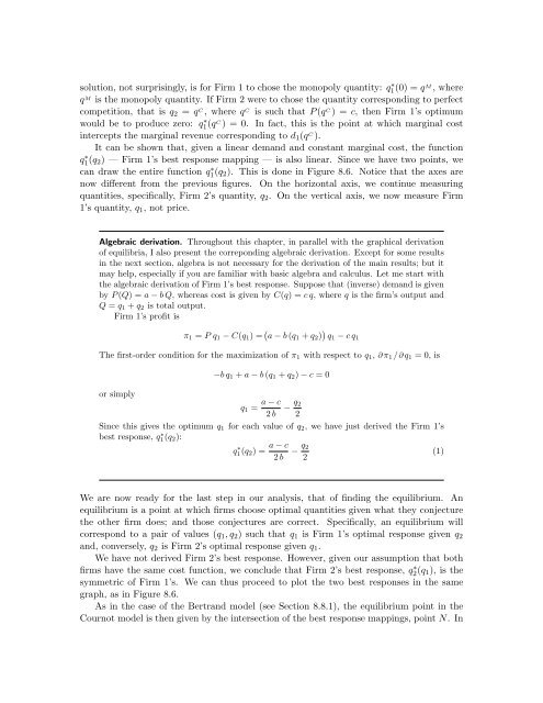
solution, not surprisingly, is for Firm 1 to chose the monopoly quantity: q1 ∗(0) = qM , where
q M is the monopoly quantity. If Firm 2 were to chose the quantity corresponding to perfect
competition, that is q 2 = q C , where q C is such that P (q C ) = c, then Firm 1’s optimum
would be to produce zero: q1 ∗(qC ) = 0. In fact, this is the point at which marginal cost
intercepts the marginal revenue corresponding to d 1 (q C ).
It can be shown that, given a linear demand and constant marginal cost, the function
q1 ∗(q 2) — Firm 1’s best response mapping — is also linear. Since we have two points, we
can draw the entire function q1 ∗(q 2). This is done in Figure 8.6. Notice that the axes are
now different from the previous figures. On the horizontal axis, we continue measuring
quantities, specifically, Firm 2’s quantity, q 2 . On the vertical axis, we now measure Firm
1’s quantity, q 1 , not price.
Algebraic derivation. Throughout this chapter, in parallel with the graphical derivation
of equilibria, I also present the correponding algebraic derivation. Except for some results
in the next section, algebra is not necessary for the derivation of the main results; but it
may help, especially if you are familiar with basic algebra and calculus. Let me start with
the algebraic derivation of Firm 1’s best response. Suppose that (inverse) demand is given
by P (Q) = a − b Q, whereas cost is given by C(q) = c q, where q is the firm’s output and
Q = q 1 + q 2 is total output.
Firm 1’s profit is
π 1 = P q 1 − C(q 1 ) = ( a − b (q 1 + q 2 ) ) q 1 − c q 1
The first-order condition for the maximization of π 1 with respect to q 1 , ∂ π 1 /∂ q 1 = 0, is
or simply
−b q 1 + a − b (q 1 + q 2 ) − c = 0
q 1 = a − c − q 2
2 b 2
Since this gives the optimum q 1 for each value of q 2 , we have just derived the Firm 1’s
best response, q1(q ∗ 2 ):
q ∗ 1(q 2 ) = a − c
2 b
− q 2
2
(1)
We are now ready for the last step in our analysis, that of finding the equilibrium. An
equilibrium is a point at which firms choose optimal quantities given what they conjecture
the other firm does; and those conjectures are correct. Specifically, an equilibrium will
correspond to a pair of values (q 1 , q 2 ) such that q 1 is Firm 1’s optimal response given q 2
and, conversely, q 2 is Firm 2’s optimal response given q 1 .
We have not derived Firm 2’s best response. However, given our assumption that both
firms have the same cost function, we conclude that Firm 2’s best response, q2 ∗(q 1), is the
symmetric of Firm 1’s. We can thus proceed to plot the two best responses in the same
graph, as in Figure 8.6.
As in the case of the Bertrand model (see Section 8.8.1), the equilibrium point in the
Cournot model is then given by the intersection of the best response mappings, point N. In