8 Oligopoly - Luiscabral.net

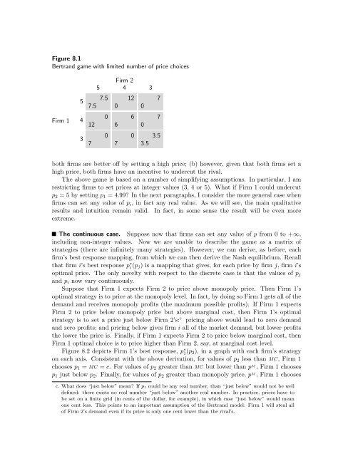
Figure 8.1
Bertrand game with limited number of price choices
Firm 1
5
4
3
Firm 2
5 4 3
7.5 12 7
7.5 0 0
0 6 7
12 6 0
0 0 3.5
7 7 3.5
both firms are better off by setting a high price; (b) however, given that both firms set a
high price, both firms have an incentive to undercut the rival.
The above game is based on a number of simplifying assumptions. In particular, I am
restricting firms to set prices at integer values (3, 4 or 5). What if Firm 1 could undercut
p 2 = 5 by setting p 1 = 4.99? In the next paragraphs, I consider the more general case when
firms can set any value of p i , in fact any real value. As we will see, the main qualitative
results and intuition remain valid. In fact, in some sense the result will be even more
extreme.
The continuous case. Suppose now that firms can set any value of p from 0 to +∞,
including non-integer values. Now we are unable to describe the game as a matrix of
strategies (there are infinitely many strategies). However, we can derive, as before, each
firm’s best response mapping, from which we can then derive the Nash equilibrium. Recall
that firm i’s best response p ∗ i (p j) is a mapping that gives, for each price by firm j, firm i’s
optimal price. The only novelty with respect to the discrete case is that the values of p j
and p i now vary continuously.
Suppose that Firm 1 expects Firm 2 to price above monopoly price. Then Firm 1’s
optimal strategy is to price at the monopoly level. In fact, by doing so Firm 1 gets all of the
demand and receives monopoly profits (the maximum possible profits). If Firm 1 expects
Firm 2 to price below monopoly price but above marginal cost, then Firm 1’s optimal
strategy is to set a price just below Firm 2’s: c pricing above would lead to zero demand
and zero profits; and pricing below gives firm i all of the market demand, but lower profits
the lower the price is. Finally, if Firm 1 expects Firm 2 to price below marginal cost, then
Firm 1 optimal choice is to price higher than Firm 2, say, at marginal cost level.
Figure 8.2 depicts Firm 1’s best response, p ∗ 1 (p 2), in a graph with each firm’s strategy
on each axis. Consistent with the above derivation, for values of p 2 less than MC , Firm 1
chooses p 1 = MC = c. For values of p 2 greater than MC but lower than p M , Firm 1 chooses
p 1 just below p 2 . Finally, for values of p 2 greater than monopoly price, p M , Firm 1 chooses
c. What does “just below” mean? If p 1 could be any real number, than “just below” would not be well
defined: there exists no real number “just below” another real number. In practice, prices have to
be set on a finite grid (in cents of the dollar, for example), in which case “just below” would mean
one cent less. This points to an important assumption of the Bertrand model: Firm 1 will steal all
of Firm 2’s demand even if its price is only one cent lower than the rival’s.