8 Oligopoly - Luiscabral.net

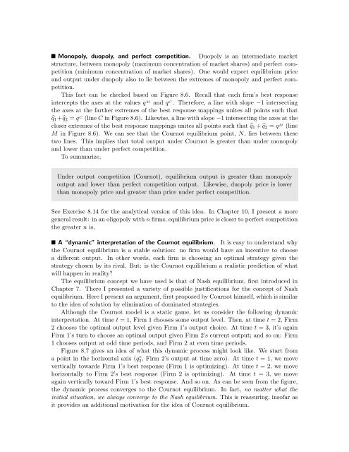
Monopoly, duopoly, and perfect competition. Duopoly is an intermediate market
structure, between monopoly (maximum concentration of market shares) and perfect competition
(minimum concentration of market shares). One would expect equilibrium price
and output under duopoly also to lie between the extremes of monopoly and perfect competition.
This fact can be checked based on Figure 8.6. Recall that each firm’s best response
intercepts the axes at the values q M and q C . Therefore, a line with slope −1 intersecting
the axes at the farther extremes of the best response mappings unites all points such that
̂q 1 +̂q 2 = q C (line C in Figure 8.6). Likewise, a line with slope −1 intersecting the axes at the
closer extremes of the best response mappings unites all points such that ̂q 1 + ̂q 2 = q M (line
M in Figure 8.6). We can see that the Cournot equilibrium point, N, lies between these
two lines. This implies that total output under Cournot is greater than under monopoly
and lower than under perfect competition.
To summarize,
Under output competition (Cournot), equilibrium output is greater than monopoly
output and lower than perfect competition output. Likewise, duopoly price is lower
than monopoly price and greater than price under perfect competition.
See Exercise 8.14 for the analytical version of this idea. In Chapter 10, I present a more
general result: in an oligopoly with n firms, equilibrium price is closer to perfect competition
the greater n is.
A “dynamic” interpretation of the Cournot equilibrium. It is easy to understand why
the Cournot equilibrium is a stable solution: no firm would have an incentive to choose
a different output. In other words, each firm is choosing an optimal strategy given the
strategy chosen by its rival. But: is the Cournot equilibrium a realistic prediction of what
will happen in reality?
The equilibrium concept we have used is that of Nash equilibrium, first introduced in
Chapter 7. There I presented a variety of possible justifications for the concept of Nash
equilibrium. Here I present an argument, first proposed by Cournot himself, which is similar
to the idea of solution by elimination of dominated strategies.
Although the Cournot model is a static game, let us consider the following dynamic
interpretation. At time t = 1, Firm 1 chooses some output level. Then, at time t = 2, Firm
2 chooses the optimal output level given Firm 1’s output choice. At time t = 3, it’s again
Firm 1’s turn to choose an optimal output given Firm 2’s current output; and so on: Firm
1 chooses output at odd time periods, and Firm 2 at even time periods.
Figure 8.7 gives an idea of what this dynamic process might look like. We start from
a point in the horizontal axis (q2 ◦ , Firm 2’s output at time zero). At time t = 1, we move
vertically towards Firm 1’s best response (Firm 1 is optimizing). At time t = 2, we move
horizontally to Firm 2’s best response (Firm 2 is optimizing). At time t = 3, we move
again vertically toward Firm 1’s best response. And so on. As can be seen from the figure,
the dynamic process converges to the Cournot equilibrium. In fact, no matter what the
initial situation, we always converge to the Nash equilibrium. This is reassuring, insofar as
it provides an additional motivation for the idea of Cournot equilibrium.