AvaRaman Operating manual AvaSoft Raman 7.3 November 2008
AvaRaman Operating manual AvaSoft Raman 7.3 November 2008
AvaRaman Operating manual AvaSoft Raman 7.3 November 2008

Create successful ePaper yourself
Turn your PDF publications into a flip-book with our unique Google optimized e-Paper software.
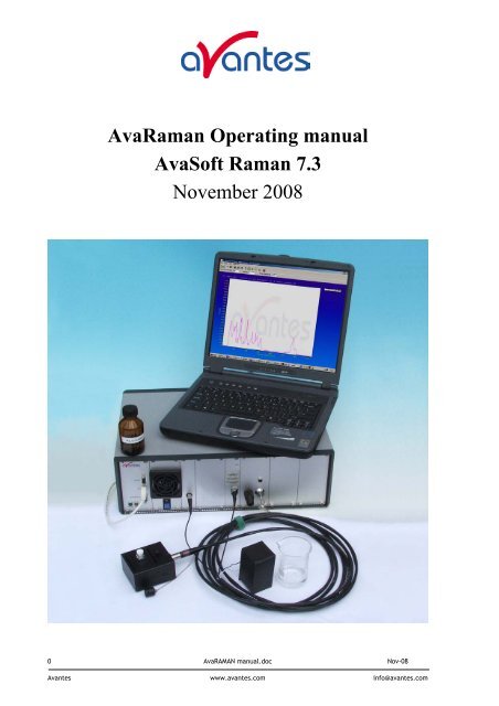
<strong>Ava<strong>Raman</strong></strong> <strong>Operating</strong> <strong>manual</strong><br />
<strong>AvaSoft</strong> <strong>Raman</strong> <strong>7.3</strong><br />
<strong>November</strong> <strong>2008</strong><br />
0 AvaRAMAN <strong>manual</strong>.doc Nov-08<br />
Avantes www.avantes.com info@avantes.com
0 SAFETY PROCEDURES AND WARNINGS 4<br />
1.0 AVARAMAN SYSTEM 6<br />
1.1 Parts included in the shipment 6<br />
1.1.1 <strong>Ava<strong>Raman</strong></strong> Spectrometer 7<br />
1.1.2 Safety Goggles 7<br />
1.1.3 Power cord 7<br />
1.1.4 USB or RS-232 interface cable 7<br />
1.1.5 AvaSpec Product CD-rom 7<br />
1.1.6 Wavelength Calibration Data Sheet 7<br />
1.1.7 <strong>Ava<strong>Raman</strong></strong> Probe 7<br />
1.2 Technical Data 8<br />
1.2.1 Technical Data Spectrometer 8<br />
1.2.2 Technical Data Laser 8<br />
1.2.3 Technical Data Probes 9<br />
1.3 Connections 11<br />
1.4 Hardware Installation 14<br />
2.0 AVASOFT INSTALLATION 15<br />
2.1 QUICK START: MEASURING AND SAVING A SPECTRUM 18<br />
2.2 MAIN WINDOW 19<br />
2.2.1 Menu bar 19<br />
2.2.2 Button bar 19<br />
2.2.3 Edit bar 21<br />
2.2.4 Graphical region 22<br />
2.2.5 Status bar 23<br />
2.2.6 Find peaks or valleys by CTRL or SHIFT + left mouse button click 24<br />
2.3 MENU OPTIONS 25<br />
2.3.1 File Menu 25<br />
2.3.1.1 File Menu: Start New Experiment 25<br />
2.3.1.2 File Menu: Load Dark 25<br />
2.3.1.3 File Menu: Load Experiment 26<br />
2.3.1.4 File Menu: Save Dark 26<br />
2.3.1.5 File Menu: Save Experiment 26<br />
Nov-08 AvaRAMAN <strong>manual</strong>.doc 1<br />
Avantes www.avantes.com info@avantes.com
2.3.1.6 File Menu: Print 27<br />
2.3.1.7 File Menu: Black and White printer 27<br />
2.3.1.8 File Menu: Display Saved Graph 27<br />
2.3.1.9 File Menu: Convert Graph - to ASCII 29<br />
2.3.1.10 File Menu: Save Graph to .RTF 29<br />
2.3.1.11 File Menu: Exit 29<br />
2.3.2 Setup Menu 30<br />
2.3.2.1 Setup Menu: Hardware 30<br />
2.3.2.2 Setup Menu: Wavelength Calibration Coefficients 30<br />
2.3.2.3 Setup Menu: Smoothing and Spline 31<br />
2.3.2.4 Setup Menu: Correct for Dynamic Dark 32<br />
2.3.2.5 Setup Menu: Subtract Saved Dark 33<br />
2.3.2.6 Setup Menu: Options 33<br />
2.3.2.6.1 Setup Menu: Options – Check on Saturation 33<br />
2.3.2.6.2 Setup Menu: Options – Full Width Half Max 36<br />
2.3.2.6.3 Setup Menu: Options - Integrals 37<br />
2.3.2.6.4 Setup Menu: Options – Autosave Spectra Periodically 38<br />
2.3.2.6.5 Setup Menu: Options – Automatic Save Dark by TTL Shutter 38<br />
2.3.2.6.6 Setup Menu: Options – Suppress Save Comments 38<br />
2.3.2.6.7 Setup Menu: Options – <strong>Raman</strong> Laser Wavelength 39<br />
2.3.2.6.8 Setup Menu: Options – Use Non-Linearity Correction 40<br />
2.3.2.6.9 Setup Menu: Options – Use Baseline Correction 40<br />
2.3.3 View Menu 42<br />
2.3.3.1 View Menu: Normalized Counts 42<br />
2.3.3.2 View Menu: Channel 44<br />
2.3.3.3 View Menu: Change Graph Scale 44<br />
2.3.3.4 View Menu: Graphic Reset 44<br />
2.3.3.5 View Menu: Autoscale Y-axis 44<br />
2.3.3.6 View Menu: Goto Preset Scale 44<br />
2.3.3.7 View Menu: Display Wavelength (nm) at X-Axis 44<br />
2.3.3.8 View Menu: Invert X-Axis 45<br />
2.3.3.9 View Menu: Grid Enable 45<br />
2.3.3.10 View Menu: Progress Bar Enable 45<br />
2.3.4 Applications: History Channel Functions 46<br />
2.3.4.1 History Application: Function Entry 46<br />
2.3.4.2 History Application: Start Measuring 51<br />
2.3.4.3 History Application: Display Saved History Graph 52<br />
2.3.5 Applications: Excel Output 54<br />
2.3.5.1 Select Source Data 54<br />
2.3.5.2 Enable Excel Output 54<br />
2.3.5.3 Settings 55<br />
2.3.5.4 Start Output 59<br />
2.3.5.5 Stop Output 59<br />
2.3.5.6 Limitations and Optimization Notes 60<br />
2.3.6 Applications: Process Control Application 61<br />
2.3.6.1 Digital Output signals 61<br />
2.3.6.2 Using the Process Control Application in <strong>AvaSoft</strong> 61<br />
2 AvaRAMAN <strong>manual</strong>.doc Nov-08<br />
Avantes www.avantes.com info@avantes.com
APPENDIX A TROUBLESHOOTING 63<br />
How to rectify an incorrect (USB) installation 63<br />
Nov-08 AvaRAMAN <strong>manual</strong>.doc 3<br />
Avantes www.avantes.com info@avantes.com
0 SAFETY PROCEDURES AND WARNINGS<br />
FOR YOUR SAFETY, READ AND UNDERSTAND ALL SAFETY AND OPERATING INSTRUCTIONS BEFORE<br />
USING THIS PRODUCT.<br />
Optical Safety<br />
The laser beam emerging from the <strong>Ava<strong>Raman</strong></strong> laser output port or from the fiber optic probe is<br />
a Class IV laser. This laser product produces visible and/or invisible laser radiation. It is<br />
capable of causing serious eye injury and blindness to anyone who looks directly into the beam<br />
or its specular reflections. Laser safety eyewear (AVARAMAN-GL-785) must be worn before<br />
applying power to the unit. Laser safety eyewear must be worn at all times while operating the<br />
<strong>Ava<strong>Raman</strong></strong>. The laser will operate at full power at 785nm within 2 seconds of applying power<br />
to the unit and it operates in continuous wave (cw) mode at 785nm with a 500mW-output<br />
power.<br />
The backside power switch controls the power to the system. When the system is on, the green<br />
Spectrometer LED will be on. The key switch on the front panel of the <strong>Ava<strong>Raman</strong></strong> labeled LASER ON<br />
| OFF controls the power to the laser. When the laser is on, the red Laser Power Indicator Lamp will<br />
be on.<br />
Due to the dangers associated with operating lasers, the AVARAMAN-GL-785 Safety Goggles are<br />
specified with every <strong>Ava<strong>Raman</strong></strong> order. It is the customer’s responsibility to supply the correct laser<br />
safety eyewear to anyone who could be exposed to the laser radiation. Reputable distributors of<br />
laser safety eyewear can recommend the best product for a user’s specific needs.<br />
Laser light presents special safety hazards not associated with other light sources. People present<br />
while a laser is in operation need to be aware of the special properties and dangers involved in laser<br />
radiation. Familiarity with the <strong>Ava<strong>Raman</strong></strong> and the properties of intense laser radiation will aid in the<br />
safe operation of this product. <strong>Ava<strong>Raman</strong></strong> users must read and understand all of the information<br />
presented in the <strong>Raman</strong> Systems <strong>Ava<strong>Raman</strong></strong> <strong>Operating</strong> Instructions before operating the <strong>Raman</strong><br />
System.<br />
The <strong>Ava<strong>Raman</strong></strong> System has following internal laser safety protection installed:<br />
1. Key-switch, please remove the key, such that unauthorized operators cannot switch on the<br />
laser<br />
2. Interlock, connect the interlock to a door switch, such that the laser is automatically<br />
switched off when the door is opened<br />
3. SMA connector micro-switch, the laser is automatically switched off when no SMA coupled<br />
fiber probe is inserted into the laser exit.<br />
4 AvaRAMAN <strong>manual</strong>.doc Nov-08<br />
Avantes www.avantes.com info@avantes.com
<strong>Ava<strong>Raman</strong></strong> users must adhere to the following regulations:<br />
1. Never look directly into the laser light source.<br />
2. Never stare at the diffuse reflected beam.<br />
3. Never sight down the beam into the source.<br />
4. Do not turn the laser on unless the fiber-optic probe is connected to the <strong>Ava<strong>Raman</strong></strong>.<br />
5. Do not disconnect the fiber-optic probe from the <strong>Ava<strong>Raman</strong></strong> unless the laser is turned off.<br />
6. Restrict the use of the <strong>Ava<strong>Raman</strong></strong> to qualified and well-trained users knowledgeable in laser<br />
safety practices. In addition, inform all personnel working in the area of these regulations.<br />
7. Before the laser is in operation, notify all personnel in the room or others who might be<br />
exposed to the laser beam that a laser is about to be used.<br />
8. Illuminate warning lights and post warning signs in the area when the laser is in operation.<br />
9. People requiring access to areas within the nominal hazard zone must wear protective eyewear<br />
designed for 785nm lasers with the 785 nm system and 532 nm with the 532 nm system. The<br />
eyewear designation should permit observation of the emission indicator.<br />
10. Position the beam path and optical components used in the operation of the <strong>Ava<strong>Raman</strong></strong> at an<br />
elevation low enough to prevent inadvertent beam-to-eye contact.<br />
11. Reflections from shiny surfaces, such as watches, rings, window glass, polished surfaces, etc.,<br />
can redirect light in dangerous directions. Whenever the laser light can possibly illuminate a<br />
shiny object, consider where the reflected light could go and make sure that a hazardous<br />
situation is not created. Even a diffused reflection of a Class IV laser product is dangerous.<br />
12. User should consult with their laser safety division, if applicable.<br />
13. Use of a Class IV laser product requires power interlocks installed on every door leading to the<br />
lab.<br />
Upgrades<br />
Customers sometimes find that they need Avantes to make a change to or to upgrade their system.<br />
In order for Avantes to make these changes, the customer must first contact us and obtain a Return<br />
Merchandise Authorization (RMA) number. Please contact the Avantes Technical Services for specific<br />
instructions when returning a product.<br />
If you still have problems with your installation, do not hesitate to contact us:<br />
Avantes Technical Support<br />
Soerense Zand Noord 26<br />
NL-6961 RB Eerbeek<br />
The Netherlands<br />
Tel. +31-(0) 313-670170, Fax. +31-(0) 313-670179<br />
www.avantes.com, info@avantes.com<br />
Nov-08 AvaRAMAN <strong>manual</strong>.doc 5<br />
Avantes www.avantes.com info@avantes.com
1.0 <strong>Ava<strong>Raman</strong></strong> System<br />
The <strong>Ava<strong>Raman</strong></strong> <strong>Raman</strong> System is a fully integrated,<br />
low-cost system for applications requiring <strong>Raman</strong><br />
techniques. The <strong>Ava<strong>Raman</strong></strong> system consists of a<br />
laser diode, an AvaSpec 2048 CCD-array<br />
spectrometer and an expanded range of fiber optic<br />
probes. The <strong>Ava<strong>Raman</strong></strong> System is available for<br />
multiple <strong>Raman</strong> wavelengths in 2 basic versions:<br />
1. The low-cost non-cooled version with 25<br />
cm –1 resolution, standard built-in solid state<br />
laser .<br />
2. The high performance, TE-cooled version<br />
with a stabilized Laser that can achieve an<br />
optical resolution of 8 cm -1 .<br />
Both <strong>Ava<strong>Raman</strong></strong> systems come with special <strong>AvaSoft</strong>-<strong>Raman</strong> software (see software section). The<br />
<strong>Ava<strong>Raman</strong></strong> System is optimized for maximum sensitivity. The maximum integration time is 60<br />
seconds.<br />
The <strong>Ava<strong>Raman</strong></strong> is especially useful for analysis, such as reaction monitoring, product identification,<br />
remote sensing, and the characterization of highly scattering particulate matter in aqueous<br />
solutions, gels and other media.<br />
The <strong>Ava<strong>Raman</strong></strong> System is also available with different Laser types than the standard 785nm, such as<br />
Ar-Ion 514 nm, solid-state 50 or 100 mW green (532 nm) lasers or HeNe lasers 633nm.<br />
1.1 Parts included in the shipment<br />
In your shipment box you will find following, please check carefully that all items are present:<br />
• <strong>Ava<strong>Raman</strong></strong> spectrometer, depending on the model a 19” rackmount or 9.5” desktop<br />
• Safety goggles (needs to be ordered separately)<br />
• Power cord (standard EUR, also –US, -UK or –AUS version available)<br />
• USB or RS-232 interface cable<br />
• <strong>Ava<strong>Raman</strong></strong> Product CD-rom<br />
• Wavelength Calibration Data Sheet<br />
• <strong>Ava<strong>Raman</strong></strong> probe (needs to be ordered separately)<br />
6 AvaRAMAN <strong>manual</strong>.doc Nov-08<br />
Avantes www.avantes.com info@avantes.com
1.1.1 <strong>Ava<strong>Raman</strong></strong> Spectrometer<br />
Depending on the model, a 19” rackmount (for the high-end <strong>Ava<strong>Raman</strong></strong>-TEC system) or 9.5”<br />
desktop.<br />
A detailed description of all connections is given in paragraph 1.2.<br />
On the backside a sticker is located with spectrometer type, serial nr, installed options date and<br />
customer name.<br />
Please follow instructions in chapter 1.4 and 2 for installation.<br />
1.1.2 Safety Goggles<br />
Safety goggles should be included in the shipment and have to worn at all times when installing the<br />
system and having the laser swiched on.<br />
1.1.3 Power cord<br />
The supplied power cord is standard equipped with EUR connection and is suitable for 100-240 VAC.<br />
If you need different socket connection, please contact us for US, UK or Australian power cords.<br />
Please follow instructions in chapter 1 or 2 before connecting the power supply.<br />
1.1.4 USB or RS-232 interface cable<br />
Standard a USB interface cable is included in the shipment. For connection under RS-232 a 9- pole<br />
IC-DB9-2 interface cable should be separately ordered with the instrument.<br />
1.1.5 AvaSpec Product CD-rom<br />
The <strong>Ava<strong>Raman</strong></strong> CD-ROM includes the installation software for the<br />
<strong>Ava<strong>Raman</strong></strong> system. It also includes a PDF version of this <strong>manual</strong> and a PDF<br />
version of the Avantes catalog.<br />
1.1.6 Wavelength Calibration Data Sheet<br />
This calibration sheet is unique to your spectrometer; it includes the<br />
wavelength calibration coefficients, installed grating, wavelength<br />
range and options as well as the spectrometer serial nr.<br />
Please make sure to save this document in a secure place.<br />
1.1.7 <strong>Ava<strong>Raman</strong></strong> Probe<br />
A number of <strong>Ava<strong>Raman</strong></strong> probes can be ordered with the <strong>Ava<strong>Raman</strong></strong><br />
system, depending on the wavelength range and application. Please<br />
see section 1.2.3 for more information.<br />
Nov-08 AvaRAMAN <strong>manual</strong>.doc 7<br />
Avantes www.avantes.com info@avantes.com
1.2 Technical Data<br />
1.2.1 Technical Data Spectrometer<br />
<strong>Ava<strong>Raman</strong></strong>-785<br />
<strong>Ava<strong>Raman</strong></strong>-785TEC<br />
Signal to noise Ratio 200:1 for Benzene 300:1 for Benzene<br />
Resolution 25 cm -1 8 cm -1<br />
Spectrometer<br />
AvaSpec-2048 with grating IB<br />
(780-1100nm), slit-50, DCL-UV/VIS<br />
AvaSpec-2048TEC with grating<br />
NC(780-930nm), slit-25, DCL-<br />
UV/VIS<br />
Spectral Range 100-2700 cm -1 (790-1050nm) 100-2100 cm -1 (785-930nm)<br />
Temperature cooled<br />
CCD<br />
n.a.<br />
Time to stabilize Depending on integration time 1-2 Minutes<br />
Dynamic Range<br />
improvement for it > 5<br />
seconds<br />
Dark Noise improvement<br />
for it > 5 seconds<br />
Peltier cooling internal<br />
Power supply<br />
n.a. > Factor 10<br />
n.a. Factor 2-3<br />
n.a.<br />
∆T = ca. -30 °C versus ambient<br />
Ca. 3.0 V, 4A<br />
External Power supply 100-240 VAC, 30W 100-240 VAC, 30W<br />
Dimensions 310 x 235 x 135 mm Desktop 320 x 450 x 135 mm Rackmount<br />
1.2.2 Technical Data Laser<br />
<strong>Ava<strong>Raman</strong></strong>-785<br />
<strong>Ava<strong>Raman</strong></strong>-785TEC<br />
Laser output (785nm) 500 mW, Class 3b 500 mW, Class 3b<br />
Laser Wavelength 785 nm 785 nm<br />
Laser Bandwidth Ca. 2.5 nm < 0.2 nm<br />
Connection 100µm, SMA905 100µm, SMA905<br />
8 AvaRAMAN <strong>manual</strong>.doc Nov-08<br />
Avantes www.avantes.com info@avantes.com
1.2.3 Technical Data Probes<br />
Since there are a variety of probes available, please find below some of the standard probes and<br />
their specifications:<br />
<strong>Ava<strong>Raman</strong></strong>-PRB-785<br />
3/8” SS low-cost focusing probe with<br />
a 90µm excitation fiber and 200µm<br />
read fiber, n.a. 0.22.<br />
Multiple focal lengths available (5<br />
mm, 7.5mm(standard), 10mm).<br />
Manual shutter included, 1.5 m<br />
cable, standard SMA905 connectors.<br />
Filter Specs OD>6 @ 785nm.<br />
Temperature up to 80°C.<br />
This probe cannot be used directly in<br />
fluids, NOT IMMERSIBLE.<br />
<strong>Ava<strong>Raman</strong></strong>-PRB-FP-785<br />
1/2" SS focusing probe with a 90µm<br />
excitation fiber and 200µm read<br />
fiber, n.a. 0.22.<br />
Multiple focal lengths available (5<br />
mm(standard), 7.5mm, 10mm).<br />
5 m cable, standard SMA905<br />
connectors.<br />
Filter Specs OD>6 @ 785nm.<br />
Temperature up to 80°C.<br />
This probe cannot be used directly in<br />
fluids, NOT IMMERSIBLE.<br />
<strong>Ava<strong>Raman</strong></strong>-PRB-FIP-785<br />
5/8" SS focusing immersible probe for<br />
in-situ measurements with a 100µm<br />
excitation fiber and 200µm read<br />
fiber, n.a. 0.22.<br />
Focal length 7.5mm (5/10mm<br />
available).<br />
5 m cable, standard SMA905<br />
connectors.<br />
Filter Specs OD>6 @ 785nm.<br />
Temperature up to 200°C.<br />
Nov-08 AvaRAMAN <strong>manual</strong>.doc 9<br />
Avantes www.avantes.com info@avantes.com
<strong>Ava<strong>Raman</strong></strong>-PRB-FC-785<br />
3/8" SS focusing process industrial<br />
probe for in-situ measurements with<br />
a 100µm excitation fiber and 200µm<br />
read fiber, n.a. 0.22.<br />
Focal length 7.5mm (5/10mm<br />
available), <strong>manual</strong> shutter.<br />
5 m cable, standard SMA905<br />
connectors.<br />
Filter Specs OD>6 @ 785nm.<br />
Temperature up to 400°C and<br />
pressure up to 200 bar.<br />
10 AvaRAMAN <strong>manual</strong>.doc Nov-08<br />
Avantes www.avantes.com info@avantes.com
1.3 Connections<br />
TEC cooling fan<br />
SMA Laser output<br />
LED laser ON<br />
Frontside<br />
RS-232 connector<br />
USB1 connector<br />
I/O connector<br />
Power LED green<br />
Scan LED yellow<br />
SMA Spectrometer<br />
Keyswitch<br />
Backside<br />
TEC switch/LED<br />
Interlock/Doorlock<br />
TEC cooling fan<br />
Power connector<br />
Fuse<br />
Switch<br />
Power LED green and scan LED yellow<br />
The green and yellow LED´s act as status LED´s for the micro controller with following meaning:<br />
Green LED = off, power is not connected<br />
Green LED = on, power is on, micro controller ready, no errors<br />
Green LED = blinking, permanent error detected by micro controller<br />
Yellow LED = on, when scan is transmitted to PC<br />
TEC switch and indicator<br />
The blue switch is used to switch on the CCD detector cooling, the green LED=on indicates that the<br />
CCD detector cooling is switched on.<br />
Switch in down position Cooling is on<br />
Switch in up position Cooling is off<br />
Nov-08 AvaRAMAN <strong>manual</strong>.doc 11<br />
Avantes www.avantes.com info@avantes.com
RS-232 connector<br />
The RS232 interface has the following physical characteristics:<br />
• 1 start bit, 8 data bits, 1 stop bit<br />
• baud rate 115200 bps<br />
• flow control with RTS/CTS<br />
• female 9 pole Sub-D connector<br />
Pin Dir Description<br />
1 out Data Carrier Detect (DTD), not connected<br />
2 out Transmit data (TX)<br />
3 in Receive data (RX)<br />
4 in Data Terminal Ready (DTR), connected to 6<br />
5 Common<br />
6 out Data Set Ready (DSR), connected to 4<br />
7 in Request To Send (RTS)<br />
8 out Clear To Send (CTS)<br />
9 out Ring Indicator, not connected<br />
USB connector<br />
The USB interface has the following physical characteristics:<br />
• USB version 1.1<br />
• high speed, 12Mbit<br />
• endpoint node, no HUB function<br />
Pin<br />
Description<br />
1 V+<br />
2 D-<br />
3 D+<br />
4 Common<br />
SMA Spectrometer<br />
This is the optical entrance that the fiber optic probe SMA connector return leg should be<br />
connected to. Please rotate SMA connector clockwise to fasten.<br />
SMA Laser output Spectrometer<br />
This is the optical exit that the fiber optic probe SMA connector illumination leg should be<br />
connected to. Please rotate SMA connector clockwise to fasten. The optical laser output is<br />
protected by a microswitch, so only when the SMA connector is fully fastened the laser will<br />
switch on.<br />
DO NOT LOOK IN THE (REFLECTED) LASER BEAM, WEAR SAFETY GOGGLES AT ALL TIMES.<br />
Interlock/doorlock<br />
For a safe operation of the instrument it is required that interlocks are connected on every door to<br />
the lab that the <strong>Raman</strong> is operated in. The delivered interlock will operate the laser without the<br />
need for interlocks on the doors, but has to be replaced by interlocks on the doors.<br />
12 AvaRAMAN <strong>manual</strong>.doc Nov-08<br />
Avantes www.avantes.com info@avantes.com
Keyswitch<br />
A keyswitch with 2 keys is delivered with the instrument, you can switch on the laser unit by<br />
rotating the key clockwise. Make sure the key is stored in a safe place, so that only authorized<br />
personel can operate the instrument.<br />
Power connector with Fuse and switch (rear panel)<br />
The power connector for 100-240 VAC is located on the rear of the AvaSpec-2048TEC. Be carefull to<br />
use for designated power range only, please use included power cord with the instrument. For UK,<br />
US and Australian power cords, contact Avantes Technical Support. The Fuse is a 2A slow blowing<br />
Fuse.<br />
Disconnect power before opening housing or replace Fuse.<br />
The installation category for this equipment is Class 2, it is not permitted to connect equipment to<br />
the <strong>Ava<strong>Raman</strong></strong> with a power supply without SELV or class II qualification.<br />
Nov-08 AvaRAMAN <strong>manual</strong>.doc 13<br />
Avantes www.avantes.com info@avantes.com
1.4 Hardware Installation<br />
1. Unpack all items and carefully check if all items, as described in 1.1 are included in the<br />
shipment.<br />
2. First install the Software on the PC, follow instructions in paragraph 2.0<br />
3. Put on the Laser Safety Goggles.<br />
4. Now connect the power cable to the backside of the <strong>Ava<strong>Raman</strong></strong> unit.<br />
5. Connect the fiberoptic probe with the corresponding legs to the SMA connector of the<br />
Spectrometer and the SMA connector of the Laser(see picture 1.3)<br />
6. Connect the probe to the experimental setup or other accessories, such as sample holder, etc.<br />
7. Switch on the power supply<br />
8. Now connect the USB cable to the PC and follow instructions under 2.0.<br />
9. Start the <strong>AvaSoft</strong>-<strong>Raman</strong> Software<br />
10. Switch on the TE Cooling, wait 1-2 Minutes until the signal stabilizes.<br />
11. Connect the Interlock/doorlock<br />
12. Insert the Key in the keyswitch and turn it on<br />
13. Now the laser (red LED) should be on.<br />
DO NOT LOOK IN THE (REFLECTED) LASER BEAM, WEAR SAFETY GOGGLES AT ALL<br />
TIMES.<br />
14 AvaRAMAN <strong>manual</strong>.doc Nov-08<br />
Avantes www.avantes.com info@avantes.com
2.0 <strong>AvaSoft</strong> Installation<br />
<strong>AvaSoft</strong>-RAMAN version <strong>7.3</strong> is a 32-bit application and can be installed under the following operating<br />
systems:<br />
• Windows 95/98/Me<br />
• Windows NT/2000/XP/Vista<br />
Installation program<br />
With each new spectrometer system, an AVANTES PRODUCT CD-ROM is included. To install <strong>AvaSoft</strong>-<br />
RAMAN from the CD-ROM, the file setup.exe on the CD-ROM needs to be executed.<br />
Installation Dialogs<br />
The setup program will check the system configuration of the computer. If no problems are<br />
detected, the first dialog is the “Welcome” dialog with some general information.<br />
In the next dialog, the<br />
destination directory for<br />
the <strong>AvaSoft</strong> software can<br />
be changed. The default<br />
destination directory is<br />
C:\<strong>AvaSoft</strong> <strong>7.3</strong>-<strong>Raman</strong>. If<br />
you want to install the<br />
software to a different<br />
directory, click the<br />
Browse button, select a<br />
new directory and click<br />
OK. If the specified<br />
directory does not exist,<br />
it will be created.<br />
In the next dialog, the<br />
name for the program<br />
manager group can be<br />
changed. The default<br />
name for this is<br />
“AVANTES Software”.<br />
After this, the “Start Installation” dialog is shown. After clicking the “next” button, the installation<br />
program starts installing files.<br />
After this, the “Start Installation” dialog is shown. After clicking the “next” button, the installation<br />
program starts installing files.<br />
During this installation, the installation program will check if the most recent USB driver has been<br />
installed already at the PC. If no driver is found, or if the driver needs to be upgraded, the Device<br />
Driver Installation Wizard is launched automatically, click Next<br />
Nov-08 AvaRAMAN <strong>manual</strong>.doc 15<br />
Avantes www.avantes.com info@avantes.com
After the drivers have been installed successfully, the dialog at the right is displayed, click Finish.<br />
After all files have been installed, the “Installation Complete” dialog shows up. Click Finish.<br />
Connecting the hardware<br />
Connect the AvaSpec-<strong>Raman</strong> to a power outlet. Switch the power to ON. Connect the USB connector<br />
to a USB port on your computer with the supplied USB cable. Windows will display the “Found New<br />
Hardware” dialog. Select the (default) option to install the software automatically, and click next.<br />
After the Hardware Wizard has completed, the following dialog is displayed:<br />
Click Finish to complete the installation.<br />
Please note that if the spectrometer is<br />
Connected to another USB port to which it has<br />
not been connected before, the “Found New<br />
Hardware Wizard” will need to install the<br />
software for this port as well.<br />
16 AvaRAMAN <strong>manual</strong>.doc Nov-08<br />
Avantes www.avantes.com info@avantes.com
Launching the software<br />
<strong>AvaSoft</strong> can be started from Windows Start Menu. Under Start-programs, the group “AVANTES<br />
Software” has been added. This group contains two icons. With the red “V” icon, <strong>AvaSoft</strong>-<strong>Raman</strong> is<br />
started. The <strong>AvaSoft</strong>-<strong>Raman</strong> help icon can be used to show this <strong>manual</strong> in pdf format.<br />
After starting <strong>AvaSoft</strong>, the dialog at the right<br />
will be shown to indicate that the USB<br />
connection has been detected (a similar<br />
dialog will be shown if the serial RS-232<br />
interface is used):<br />
If more than one AvaSpec spectrometer is connected to your PC, the<br />
dialog at the right will be shown which allows you to select the<br />
spectrometer serial number for which you want to use <strong>AvaSoft</strong>. Multiple<br />
spectrometers can be operated simultaneously, just by restarting <strong>AvaSoft</strong><br />
multiple times.<br />
After clicking the OK button, the main window is displayed. Refer to section 2.2 for a description<br />
about the main window components. A “Quick Start” can be found in section 2.1, if you want to<br />
start measuring immediately. Detailed information about the menu options is found in section 2.3.<br />
Depending on the extra add-on modules that were ordered for your spectrometer, three<br />
applications are available in <strong>AvaSoft</strong>, which are described in sections 2.3.4 to 2.3.6:<br />
• History (standard in <strong>AvaSoft</strong> FULL)<br />
• Process Control (add-on module)<br />
• Excel Output (add-on module)<br />
Nov-08 AvaRAMAN <strong>manual</strong>.doc 17<br />
Avantes www.avantes.com info@avantes.com
2.1 Quick Start: Measuring and saving a spectrum<br />
1. After starting <strong>AvaSoft</strong> <strong>Raman</strong>, the green Start button needs to be clicked to start measuring.<br />
2. Connect the probe to the laser and to the Spectrometer input port(s).<br />
3. Adjust the Smoothing Parameters in the Setup menu to optimize smoothing for the Fiber/Slit<br />
diameter that is used. In most <strong>Raman</strong> systems, the slit is 25 micron, and the smoothing<br />
parameter should be set to 0. Setting the smoothing parameter to 1 will show a smoother<br />
spectrum against the price of a little less resolution (see also section 3.2.3)<br />
4. Before switching on the laser, be sure to avoid direct eye contact via the probe tip. Turn on the<br />
laser. Usually some sort of spectrum may be seen on the screen. A lot of experiments with a<br />
<strong>Raman</strong> system require a long integration time, e.g. 10000 milliseconds for ethanol<br />
measurements. The integration time can be changed in the main window, in the white box<br />
below the start/stop button. If <strong>AvaSoft</strong> is collecting data, the start/stop button shows a red<br />
‘stop’ and the integration time box is gray, indicating that it cannot be changed. After clicking<br />
the ‘stop’ button the data acquisition stops and the integration time can be changed. The result<br />
of the changed integration time can be viewed after clicking the green ‘start’ button. Note that<br />
the maximum integration time for the <strong>Ava<strong>Raman</strong></strong> without additional cooler is about 30 seconds.<br />
The maximum integration time for the TE cooled <strong>Ava<strong>Raman</strong></strong>-TEC is about 65 seconds.<br />
5. When a good spectrum is displayed, turn off the laser.<br />
6. Now save the Dark data. This is be done by File-Save-Dark from the menu or by clicking the<br />
black square on the left top of the screen with the mouse. Always use Save Dark after the<br />
integration time has been changed.<br />
7. Turn on the laser again. Subtract the dark data that has been saved by clicking the ‘Subtract<br />
Saved Dark’ button, next to the dark button. To have a better look at the amplitude versus<br />
wavelength, the cursor button can be clicked. A vertical line is displayed in the graph. If the<br />
mouse cursor is placed nearby this line, the shape of the mouse cursor changes from an arrow<br />
to a ‘drag’ shape. If this shape is displayed, the left mouse button can be used to drag (keep<br />
left mouse button down) the line with the mouse towards a new position. Moving this line shows<br />
the corresponding values of wavelength and amplitude in the main screen. By clicking the red<br />
stop button, the data acquisition is stopped and the last acquired spectrum is shown in static<br />
mode. The data acquisition can be started again by clicking the same button, which now shows<br />
a green ‘Start’.<br />
8. To save the spectrum, choose File-Save-Experiment from the menu, or click the Save<br />
Experiment button from the button bar.<br />
9. Other options to save a spectrum can be found under Setup-Options-Autosave Spectra<br />
Periodically. With this option, spectra can be saved automatically according to instructions<br />
entered in "Time delay before first scan", "Time delay between scans" and “Number of scans to<br />
save”.<br />
10. To improve the Signal/Noise ratio, a number of spectra may be averaged. To do this, the value<br />
in the white average box in the main window (next to integration time) can be increased. The<br />
value can only be changed in static mode. When <strong>AvaSoft</strong> is acquiring data, the average box<br />
becomes gray.<br />
18 AvaRAMAN <strong>manual</strong>.doc Nov-08<br />
Avantes www.avantes.com info@avantes.com
2.2 Main Window<br />
2.2.1 Menu bar<br />
The menu’s and submenu’s are described in section 3.<br />
2.2.2 Button bar<br />
Start/Stop button<br />
The Start/Stop button can be used to display data real-time or to take a snapshot<br />
Cursor button<br />
After clicking the cursor button, a vertical line is displayed in the graph. If the mouse cursor is<br />
placed nearby this line, the shape of the mouse cursor changes from an arrow to a ‘drag’ shape. If<br />
this shape is displayed, the left mouse button can be used to drag (keep left mouse button down)<br />
the line with the mouse towards a new position. Moving this line shows the corresponding values of<br />
wavelength and amplitude in the main screen. As an alternative for dragging the line, the small step<br />
and big step arrow buttons may be used, or the left and right arrow keys on the keyboard. The step<br />
size for the arrow buttons can be changed by holding down the CTRL-key while clicking at a (single<br />
or double) arrow button.<br />
Save Dark button<br />
This is the black button at the left top of the screen. It needs to be clicked to save the dark data.<br />
The same result can be achieved with the option File-Save Dark.<br />
Subtract Saved Dark button<br />
After Dark data has been saved or loaded, the subtract saved dark button becomes enabled. After<br />
clicking this button, the dark spectrum will be subtracted from the measured data. The same result<br />
can be achieved by selecting the “Subtract Saved Dark” menu option under the setup menu.<br />
Save experiment button<br />
By clicking the Save Experiment button an experiment is saved. The same result can be achieved<br />
with the option File-Save Experiment.<br />
Nov-08 AvaRAMAN <strong>manual</strong>.doc 19<br />
Avantes www.avantes.com info@avantes.com
Print button<br />
By clicking the Print button a graph that is displayed on the monitor will be printed. The same<br />
result can be achieved with the option File-Print.<br />
Channel button<br />
After clicking this button, a dialog is shown in which the channels to be displayed can be selected.<br />
Since current <strong>Raman</strong> Systems are available with only one Master channel, this option can be used<br />
only to switch the online Master spectra off. Switching off may be helpful if you want to display only<br />
graphs that were saved before (File-Display Saved Graph), without the online measured data for the<br />
Master channel.. The same result can be achieved with the option View-Channel.<br />
Autoscale Y-axis button<br />
By clicking this button, the graph will be rescaled on-line. A maximum signal will be shown at about<br />
75% of the vertical scale. The same result can be achieved with the option View-Autoscale Y-axis<br />
Change Graph Scale button<br />
By clicking this button, a dialog will be shown in which the range can be changed for both X- and Y-<br />
axis. This range can be saved as well and restored any time by clicking the Goto Preset Scale button<br />
(see below). The menu option with the same functionality is View-Change Graph Scale.<br />
Goto Preset Scale button<br />
By clicking this button, the scale for X- and Y-axis will be set to a range that has been set before.<br />
The same result can be achieved with the menu option View-Goto Preset Scale<br />
Graphic Reset button<br />
By clicking this button, the X- and Y-axis will be reset to their default values. . The same result can<br />
be achieved with the option View-Graphic Reset<br />
H.C.F. button<br />
The History Channel Function button allows you to switch directly to the history channel function<br />
screen to start measuring immediately. Of course first the functions need to be defined.<br />
20 AvaRAMAN <strong>manual</strong>.doc Nov-08<br />
Avantes www.avantes.com info@avantes.com
2.2.3 Edit bar<br />
When <strong>AvaSoft</strong> is acquiring data, the edit fields are gray and non-editable. By clicking the red STOP<br />
button, data acquisition is stopped and the edit fields become white and editable. The edit bar<br />
shows the following parameters:<br />
Integration time[ms]<br />
This option changes the CCD readout frequency and therefore the exposure- or integration time of<br />
the CCD detector. The longer the integration time, the more light is exposed to the detector during<br />
a single scan, so the higher the signal. If the integration time is set too long, too much light reaches<br />
the detector. The result is that, over some wavelength range, the signal extends the maximum<br />
counts (16383) or in extreme case shows as a straight line at any arbitrary height, even near zero.<br />
Entering a shorter integration time can usually solve this.<br />
Average<br />
With this option, the number of scans to average can be set. A spectrum will be displayed after<br />
every # scans. This spectrum is the average of the # scans.<br />
<strong>Raman</strong> Shift[cm -1 ] or Wavelength[nm]<br />
The wavelength shows the position of the cursor, which becomes visible if the cursor button is<br />
down. The amplitude of the signal, which is given in the statusbar at the bottom of the main<br />
window, is the amplitude at the wavelength shown in this field.<br />
Default, the spectral data are shown versus <strong>Raman</strong> Shift in cm -1 . After the menu option ‘View -<br />
Display wavelength (nm) at X-axis’ is clicked, the wavelength in nanometers is shown at the X-axis<br />
and the <strong>Raman</strong> Shift[cm -1 ] in the edit bar changes to Wavelength [nm]:<br />
Nov-08 AvaRAMAN <strong>manual</strong>.doc 21<br />
Avantes www.avantes.com info@avantes.com
2.2.4 Graphical region<br />
The graphical region displays the data in an XY-diagram, with at the X-axis (default) the <strong>Raman</strong><br />
Shift in cm -1 , and at the Y-axis the detector counts.<br />
Display saved Graph and Line style editor<br />
By clicking on the legenda with the right mouse button, multiple spectra, that were saved earlier<br />
can be displayed.<br />
New in <strong>AvaSoft</strong> 7 is that displayed graphs can be deleted or<br />
properties of the displayed graphs, such as line style or color or<br />
comments can be changed. This is done by clicking with the right<br />
mouse button on the line in the graphical display. A small line edit<br />
box will occur.<br />
Now the line can be deactivated or the line properties can<br />
be changed as depicted in the border editor or the<br />
comments can be edited.<br />
22 AvaRAMAN <strong>manual</strong>.doc Nov-08<br />
Avantes www.avantes.com info@avantes.com
Zoom features<br />
Zoom in: select a region to be expanded to the full graph. To select this region, click the left<br />
mouse button in the white graphical region and drag it downwards and to the right. After releasing<br />
the left mouse button within the graphic display, both the X- and Y-axis will be rescaled to the new<br />
values of the selected region.<br />
Zoom out: drag with the left mouse button within the white rectangle, but in stead of dragging the<br />
mouse downwards and to the right, drag it into another direction. After releasing the mouse button,<br />
both the X- and Y-axis will be reset to their default values.<br />
Move X-Y: dragging with the right mouse button results in moving the complete spectrum up or<br />
down and to the left or right.<br />
Move-Y: if a mouse-wheel is available on the mouse being used, then the spectrum can be moved<br />
up or down by moving the mouse wheel.<br />
2.2.5 Status bar<br />
For each selected spectrometer channel, a statusbar at the bottom of the main window shows<br />
information about the file to which the data will be saved, amplitude at current wavelength, and<br />
the current settings for the smoothing and spline parameters. The field at the right of the Spline<br />
setting is used to indicate that the spectrometer is receiving too much light at a certain wavelength<br />
range (=16383 counts before correcting for dynamic dark, smoothing or averaging), in which case<br />
the label “saturated” will become visible. See also section 3.2.6.1: check on saturation.<br />
Nov-08 AvaRAMAN <strong>manual</strong>.doc 23<br />
Avantes www.avantes.com info@avantes.com
2.2.6 Find peaks or valleys by CTRL or SHIFT + left mouse button click<br />
This option can be used for all displayed graphics. When the left mouse button is clicked in the<br />
graphical region, while the CTRL key is down, <strong>AvaSoft</strong> will follow the following procedure to run to<br />
the closest peak:<br />
1. The wavelength is determined from the position the mouse click occurred.<br />
2. The data from closest pixel is retrieved<br />
3. The direction to search for the peak is determined from the neighbor pixels. If both neighbor<br />
pixels have a lower value at the Y-axis than the current pixel, the current pixel is already a<br />
peak. If only one of the neighbor pixel values is higher then the current pixel value, the peak<br />
will be searched in the direction of this higher pixel. If both neighbor pixels have a higher value<br />
at the Y-axis than the current pixel, the current pixel is in a valley. The peak will in this case be<br />
searched in the direction of this neighbor pixel with the highest value.<br />
4. The cursor starts moving in the direction, as determined under 3), until it reaches a pixel of<br />
which the value is not higher than the last one evaluated. At this pixel the cursor stops.<br />
By holding down the SHIFT key instead of the CTRL key, the same procedure will be used to move to<br />
the closest valley.<br />
If more than one spectrum is being displayed, a dialog, as shown at the<br />
right, pops up in which the spectrum for which the peakfinder needs to<br />
be activated can be selected out of all displayed spectra.<br />
24 AvaRAMAN <strong>manual</strong>.doc Nov-08<br />
Avantes www.avantes.com info@avantes.com
2.3 Menu Options<br />
In sections 3.1 to 3.3 the three main menu options (File, Setup and View) and their submenu's are<br />
described in detail. The applications menu (History, Process Control, Excel) are described in<br />
sections 3.4 to 3.6.<br />
2.3.1 File Menu<br />
2.3.1.1 File Menu: Start New Experiment<br />
After selecting this option, a dialog box appears in which a new experiment name can be entered.<br />
The experiment name will be saved as a filename with the extension *.kon. This extension does not<br />
need to be entered.<br />
After clicking the save button, the<br />
current filename will be built up from<br />
the experiment name that has been<br />
entered, and a sequence number,<br />
starting at 0001.<br />
Example: if the experiment name is<br />
TOP, the first graphic file that will be<br />
saved in scope mode, will be called<br />
TOP0001.ROH, the sequence number<br />
will be automatically incremented, so<br />
the next file that will be saved in<br />
scope mode will be called<br />
TOP0002.ROH etc. For detailed<br />
information on graphic filenames, see<br />
File-Save Experiment. Note that the dialog allows you to select different folders or drives to save<br />
the experiments to, as well as creating a new folder name for the new experiment.<br />
After closing the dialog box by clicking the save button, the new experiment name, followed by its<br />
sequence number, is displayed in the lower left of the status bar. By clicking the cancel button, the<br />
old experiment name will be restored.<br />
2.3.1.2 File Menu: Load Dark<br />
With this option, dark data can be loaded, that have been saved before. If <strong>AvaSoft</strong> is in static mode,<br />
the dark data that will be loaded are shown on the screen first.<br />
Nov-08 AvaRAMAN <strong>manual</strong>.doc 25<br />
Avantes www.avantes.com info@avantes.com
2.3.1.3 File Menu: Load Experiment<br />
With this option, an experiment can be<br />
loaded, that has been used before. This<br />
way more spectra can be saved to an<br />
existing experiment. An experiment<br />
name has the file extension "*.kon".<br />
After choosing this option, a dialog box<br />
shows all experiments that were saved<br />
earlier in the current experiment<br />
directory. If the experiment name that<br />
needs to be loaded is in this directory,<br />
select it and click the save button. If<br />
the experiment name that needs to be<br />
loaded is in another drive and/or<br />
directory, move to this directory by<br />
clicking the behind the current<br />
foldername. For detailed information on graphic filenames, see File-Save Experiment.<br />
2.3.1.4 File Menu: Save Dark<br />
With this option, dark data are saved. The name of the dark data file is "dark0.dat". The dark data<br />
files will be saved in the experiment directory that has been picked by the option File-Load-<br />
Experiment or File-Start New-Experiment.<br />
2.3.1.5 File Menu: Save Experiment<br />
With this option, spectral data is saved. All graphic files will be saved in the experiment directory<br />
that has been picked by the option File-Load-Experiment or File-Start New-Experiment.<br />
First, a window appears in which a line of comments can be entered to the saved graph. Next two<br />
files will be saved: the first file contains the saved spectrum data. The name of this first file starts<br />
with the experiment name, directly followed by the sequence number of the saved spectrum. The<br />
extension of this first file is *.ROH<br />
The second file contains the line of comments, which may have been added to this graph. The name<br />
of this second file is, except for the extension, the same as the name of the first file (experiment<br />
name and sequence number). The extension of this second file is *.RCM<br />
Example: suppose the name of our experiment is "top". Then, saving two spectra, results in the<br />
following files: top0001.roh, top0001.rcm, top0002.roh, top0002.rcm<br />
26 AvaRAMAN <strong>manual</strong>.doc Nov-08<br />
Avantes www.avantes.com info@avantes.com
After leaving the application and opening <strong>AvaSoft</strong> the next time, saving a new spectrum will then<br />
result in respectively the data-files top0003.roh and top003.rcm.<br />
Before saving, the name of the graphic file is displayed in the statusbar at the bottom of the<br />
screen. After saving, the sequence number is automatically incremented by one.<br />
2.3.1.6 File Menu: Print<br />
After selecting the print menu<br />
option, the background colors in the<br />
graphical region will become white.<br />
If the menu option “Black and White<br />
printer” (see next section) has been<br />
marked, the line style for the<br />
spectra will also change from<br />
colored to black. A dialog will be<br />
shown in which the title for the<br />
printout can be entered. In the next<br />
window, the printer settings can be<br />
changed (e.g. portrait or landscape<br />
printing, printing quality etc.). After<br />
clicking OK in the printer settings<br />
dialog, the graph will be printed,<br />
and the original graph colors will be restored on the monitor.<br />
2.3.1.7 File Menu: Black and White printer<br />
The default setting in <strong>AvaSoft</strong> is to print the spectra in the same color as they appear on the<br />
monitor. However, if a color printer is not available, the menu option “Black and White printer” can<br />
be enabled. If this option is enabled, different line styles will be printed if more than one spectrum<br />
is displayed, e.g. dash-dash, dot-dot, dash-dot. To enable this option, click the menu option and a<br />
checkmark appears in front of it.<br />
2.3.1.8 File Menu: Display Saved Graph<br />
This option requires that graphic files were<br />
saved earlier by using the option File-Save<br />
Experiment. After choosing this option, a<br />
window shows all files that were saved<br />
before.<br />
If a graphic file is marked by a (single)<br />
mouse click on the filename, the comment<br />
line for this file appears at the top of the<br />
graphical region in the main window.<br />
Selecting multiple filenames can be realized<br />
by using the CTRL or SHIFT key in<br />
combination with the mouse. If the CTRL<br />
key is pressed, all the files that are clicked by the mouse will be selected for displaying. If the<br />
SHIFT key is pressed, all the files in between two clicked files will be selected for displaying.<br />
Nov-08 AvaRAMAN <strong>manual</strong>.doc 27<br />
Avantes www.avantes.com info@avantes.com
Select the name of the file(s) to be displayed and click the Open button. To leave this dialog<br />
without displaying graphic files, click the CANCEL button.<br />
In the figure at the<br />
right, two graphic files<br />
were selected in scope<br />
mode. The comments<br />
that were saved with<br />
these graphs are<br />
displayed at the top of<br />
the graphical region,<br />
together with<br />
information about<br />
amplitude at current<br />
wavelength (amp),<br />
integration time (it)<br />
and smoothing (s)<br />
settings at the moment<br />
that the file was saved<br />
and the name of the<br />
graphic file. If the<br />
active spectrometer<br />
channel (Master) has<br />
not been unselected<br />
with the View Channel option, the actual data for the Master channel will be displayed in the same<br />
graph as the selected graphic files. By clicking the green start button, the online measurements can<br />
be compared directly to the graphics that were saved before.<br />
New in <strong>AvaSoft</strong> 7 is that displayed graphs can be deleted or<br />
properties of the displayed graphs, such as line style or color or<br />
comments can be changed. This is done by clicking with the right<br />
mouse button on the line in the graphical display. A small line<br />
edit box will occur.<br />
Now the line can be deactivated or the line properties can<br />
be changed as depicted in the border editor or the<br />
comments can be edited.<br />
The menu option File-Display Saved Graph is preceded by<br />
a checkmark as long as the earlier saved graphics are displayed. To clear these earlier saved<br />
graphics, select again the menu option File-Display Saved Graph, after which the checkmark<br />
disappears, and only the spectra for the active spectrometer channel(s) will be displayed.<br />
28 AvaRAMAN <strong>manual</strong>.doc Nov-08<br />
Avantes www.avantes.com info@avantes.com
2.3.1.9 File Menu: Convert Graph - to ASCII<br />
This option requires that graphic files were<br />
saved earlier by using the option File-Save<br />
Experiment. After choosing this option, a<br />
window shows all files that were saved<br />
before<br />
If a graphic file is marked by a (single)<br />
mouse click on the filename, the comment<br />
line for this file appears at the top of the<br />
graphical region in the main window.<br />
Selecting multiple filenames can be<br />
realized by using the CTRL or SHIFT key in<br />
combination with the mouse.<br />
If the CTRL key is pressed, all the files that are clicked by the mouse will be selected for<br />
conversion. If the SHIFT key is pressed, all the files in between two clicked files will be selected for<br />
conversion.<br />
Select the name of the file(s) to be converted to ASCII and click the Open button. To leave this<br />
dialog without converting files, click the CANCEL button. The extension of the text files wil be<br />
*.TRT.<br />
All text files start with a header with information for the graphic file that has been converted. The<br />
header shows:<br />
- the comment line<br />
- the integration time<br />
- the number of scans that has been averaged<br />
- the number of pixels used for smoothing<br />
- the serialnumber of the spectrometer that was used to save the data<br />
The data in a *.TRT file is given in three columns, separated by a “;”. The first column gives the<br />
wavelength in nanometers, the second the corresponding <strong>Raman</strong> Shift in cm -1 and the third column<br />
the detector counts at that wavelength / <strong>Raman</strong> Shift.<br />
2.3.1.10 File Menu: Save Graph to .RTF<br />
This option allows you to save the graph to a file in Rich Text File (.RTF) format. After clicking this<br />
menu option, a comment can be added and the filename can be entered in a standard Windows<br />
“Save As” dialog.<br />
2.3.1.11 File Menu: Exit<br />
Closes <strong>AvaSoft</strong>.<br />
Nov-08 AvaRAMAN <strong>manual</strong>.doc 29<br />
Avantes www.avantes.com info@avantes.com
2.3.2 Setup Menu<br />
2.3.2.1 Setup Menu: Hardware<br />
This menu option displays a list of AvaSpec serial numbers that<br />
are connected to the PC’s USB port(s) and COM port(s) and which<br />
are not used by another (instance of the) application. This option<br />
can be used to allocate a spectrometer to an application (for<br />
example if one spectrometer is running with <strong>AvaSoft</strong>-Full and<br />
another spectrometer needs to run with <strong>AvaSoft</strong>-<strong>Raman</strong><br />
software). But it can also be used to run multiple spectrometers<br />
simultaneously, just by restarting <strong>AvaSoft</strong> multiple times.<br />
After clicking the OK button, <strong>AvaSoft</strong> will communicate with the<br />
spectrometer serial number that has been activated in the<br />
dialog.<br />
2.3.2.2 Setup Menu: Wavelength Calibration Coefficients<br />
After clicking this option, a dialog is shown in which the wavelength calibration coefficients can be<br />
changed <strong>manual</strong>ly.<br />
Background<br />
The wavelength λ that corresponds to a pixel number (pixnr) in the detector in the spectrometer<br />
can be calculated by the following equation:<br />
λ = Intercept + X1*pixnr + X2*pixnr 2 + X3*pixnr 3 + X4*pixnr 4<br />
30 AvaRAMAN <strong>manual</strong>.doc Nov-08<br />
Avantes www.avantes.com info@avantes.com
in which Intercept and X1<br />
to X4 correspond to<br />
Intercept and First to<br />
Fourth Coefficient in the<br />
figure at the right. For<br />
example, if we want to<br />
calculate the wavelength at<br />
pixel number 1000, using<br />
the numbers in the figure<br />
at the right, the<br />
wavelength becomes:<br />
λ = 384,054 +<br />
0,136492*1000 +<br />
-6,71259E-6*1E6 +<br />
-5,66234E-10*1E9<br />
= 513,267 nm.<br />
The ‘Restore Factory Settings’ button restores for all spectrometer channels the original wavelength<br />
calibration coefficients that were saved to the EEPROM during factory calibration.<br />
The “Process data only when in following wavelength range” option can be used to transfer only a<br />
limited number of pixels from the spectrometer to the PC. This can significantly speed up the<br />
transfer time (e.g. for the AvaSpec-2048 from 30 ms at full wavelength down to 14 ms for a small<br />
selection of 10 pixels). A second advantage is data reduction, because only the spectral data will be<br />
saved at the pixels for which the wavelength is in the specified wavelength range.<br />
2.3.2.3 Setup Menu: Smoothing and Spline<br />
The Cubic Spline Interpolation Algorithm can be applied to<br />
get a better estimation for the spectral data between the<br />
pixels on the detector array.<br />
Smoothing is a procedure, which averages the spectral data<br />
over a number of pixels on the detector array. For example,<br />
if the smoothing parameter is set to 2, the spectral data for<br />
all pixels x n on the detector array will be averaged with their<br />
neighbor pixels x n-2 , x n-1 , x n+1 and x n+2 .<br />
Cubic Spline Interpolation<br />
In the figure below, the effect of spline interpolation is illustrated. The Master data shows the AD<br />
counts for 4 pixels, connected by a straight line (linear interpolation). The Slave1 data is for these 4<br />
pixels exactly the same as for the Master data, but this time the cubic spline interpolation<br />
algorithm has been applied, resulting in data which is smooth in the first derivative and continuous<br />
in the second derivative.<br />
Nov-08 AvaRAMAN <strong>manual</strong>.doc 31<br />
Avantes www.avantes.com info@avantes.com
The spline interpolation can be<br />
useful for applications in which<br />
the output of line sources, like<br />
laser diodes is displayed, or for<br />
other applications, which<br />
require a high resolution. Note<br />
that for the AvaSpec-2048 with<br />
2048 pixels, the effect of<br />
spline interpolation is not<br />
visible if the data is shown at<br />
full scale. The monitor<br />
resolution is much less than<br />
2048 pixels. The effect of<br />
spline interpolation can only<br />
be visualized if the number of<br />
detector pixels that are<br />
displayed is smaller than the<br />
number of monitor pixels at<br />
the x-axis.<br />
Smoothing<br />
To get a smoother spectrum without losing information it is important to set in the software the<br />
right smoothing parameter. The optimal smoothing parameter in a standard <strong>Ava<strong>Raman</strong></strong> system with<br />
50 micron slit is 1, in which case the data at each pixel will be averaged with one neighbor pixel at<br />
the left and one at the right. This can be done without losing resolution, because the 50 micron<br />
beam will cover at least 3 detector pixels (the distance between the pixels at the CCD detector is<br />
14 micron). The <strong>Ava<strong>Raman</strong></strong>-TEC includes a 25 micron slit in which case the smoothing should be set<br />
to zero.<br />
If resolution is not an important issue, a higher smoothing parameter can be set to decrease noise<br />
against the price of less resolution.<br />
2.3.2.4 Setup Menu: Correct for Dynamic Dark<br />
The pixels of the CCD detector (AvaSpec-2048) are thermally sensitive, which causes a small dark<br />
current, even without light exposure. To get an approximation of this dark current, the signal of the<br />
first 14 optical black pixels of the CCD-detector can be taken and subtracted from the raw scope<br />
data. This will happen if the correct for dynamic dark option is enabled. As these 14 pixels have the<br />
same thermal behaviour as the active pixels, the correction is dynamic.<br />
If this menu option is preceded by a checkmark, the scope data is corrected with the dynamic dark<br />
algorithm. It is recommended to leave this setting checked, which is the default state.<br />
32 AvaRAMAN <strong>manual</strong>.doc Nov-08<br />
Avantes www.avantes.com info@avantes.com
2.3.2.5 Setup Menu: Subtract Saved Dark<br />
This option is used to subtract the dark spectrum that has been saved (File-Save Dark) from the raw<br />
scope data. After starting up <strong>AvaSoft</strong>, this menu option is always unselected, because a dark<br />
spectrum needs to be saved or loaded before it can be subtracted.<br />
If this menu option is preceded by a checkmark, the scope data is corrected with the saved dark.<br />
2.3.2.6 Setup Menu: Options<br />
2.3.2.6.1 Setup Menu: Options – Check on Saturation<br />
The 14-bit A/D converter in the AvaSpec results in raw Scope pixel values between 0 and 16383<br />
counts. If the value of 16383 counts is measured at one or more pixels, then these pixels are called<br />
to be saturated or overexposed. Since saturated pixels can disturb the measurement results, a lot of<br />
attention has been given in <strong>AvaSoft</strong> (and the driver package as161.dll) to detect saturation and to<br />
notify the user if a measurement contains saturated pixels. This notification is done in such a way<br />
that the user can always decide to ignore the saturation, for example if the saturation happens at<br />
pixels that are not in the wavelength range where the user is interested in. Saturation can usually<br />
be solved by selecting a shorter integration<br />
time. In <strong>AvaSoft</strong>, different levels of saturation<br />
detection can be set, and there are also<br />
different options for notification, as shown in<br />
the figure at the right.<br />
Saturation detection levels<br />
The default level of saturation detection is<br />
“Detect Saturated Pixels at saturation level”.<br />
The third (autocorrect inverted pixels) level<br />
has been implemented to be able to correct<br />
heavily saturated pixels (at a light intensity of<br />
approximately 5 times the intensity at which<br />
saturation starts). These pixels will return<br />
values
heavily saturated peaks, the autocorrect can be used. To illustrate this, a strong peak from the<br />
AvaLight-CAL calibration line source was heavily saturated at 435.84 nm. This caused the most<br />
heavily saturated pixels to return inverted (
Additional information about the saturated wavelength ranges can be visualized and/or saved by<br />
enabling the following options:<br />
Visualize saturated pixels areas in graph<br />
By enabling this option, the spectrum in the main window will be displayed with a thicker line for<br />
these wavelength ranges where the saturation occurs. In time series measurements, the function<br />
output values that were calculated using saturated data are marked with a black dot.<br />
Log saturated pixel areas to screen<br />
By enabling the second option, a small window appears in which the<br />
spectrometer channel number (0 = Master, 1 = Slave1 etc…) and <strong>Raman</strong> Shift<br />
for the saturated pixels are given.<br />
Log saturated pixel areas to file on “Save Measurement”<br />
The third option can be used to create a file to which the saturated <strong>Raman</strong> Shift ranges will be<br />
written when a measurement is saved in <strong>AvaSoft</strong>. When saving spectra in the main window (Save<br />
button, or menu option File-Save-Experiment), the name of the logfile becomes equal to the<br />
experimentname, but with the extension *.sat. For example if a graph in absorbance mode is saved<br />
to test0001.abs and if this spectrum contains saturated data, then additional lines will be written to<br />
the textfile test.sat.<br />
If time series measurements are saved to file, the data will also be checked on saturation and if<br />
saturation occurs, additional lines will be written to a logfile with the same filename as the<br />
measurement results, but with the extension *.sat (e.g. History.sat).<br />
The files with extension *.sat can be openend with any textfile editor, for example Notepad.<br />
Nov-08 AvaRAMAN <strong>manual</strong>.doc 35<br />
Avantes www.avantes.com info@avantes.com
2.3.2.6.2 Setup Menu: Options – Full Width Half Max<br />
The Full Width Half Maximum of a peak is the bandwidth for which the intensity is higher than half<br />
of the maximum intensity of that peak. The unit for FWHM is cm -1 if the <strong>Raman</strong> Shift is displayed at<br />
the X-Axis and nanometer if the wavelength is displayed at the X-axis. This utility is used mostly<br />
measuring the output of laser diodes. During FWHM<br />
calculations, the intensity needs to be corrected for<br />
the dark data. Therefore it is recommended to<br />
enable the option Subtract Saved Dark, as shown in<br />
the dialog at the right, which appears after clicking<br />
the FWHM option. After clicking the OK button, the<br />
Full Width Half Max can be calculated for a number<br />
of peaks.<br />
To mark a peak for which the FWHM values needs to be calculated, press the ALT key, and click<br />
with the left mouse button on this peak. If only one spectrometer channel is enabled, and there are<br />
no earlier saved graphs being displayed, then the FWHM value of the marked peak will be shown<br />
directly on top of the peak. Further on, this peak will be yellow marked over the width of the FWHM<br />
value (it may be necessary to zoom in on the peak to be able to view that the peak is marked).<br />
If more than one spectrum is being displayed, a dialog, as shown at the<br />
right, pops up in which the spectrum for which the FWHM needs to be<br />
activated can be selected out of all displayed spectra.<br />
In the figure below, two peaks have been selected for FWHM<br />
calculation: one for the Master channel and one for<br />
“AVANTES0001.roh”, which is an earlier saved spectrum.<br />
The FWHM values are given in<br />
the same color as the<br />
spectrum is drawn.<br />
To disable the FWHM<br />
calculation, the menu option<br />
(which is marked as long as<br />
the FWHM is enabled), needs<br />
to be reselected.<br />
36 AvaRAMAN <strong>manual</strong>.doc Nov-08<br />
Avantes www.avantes.com info@avantes.com
2.3.2.6.3 Setup Menu: Options - Integrals<br />
This utility can be used for measuring the total amount of energy coming into the spectrometer. Up<br />
to 10 integrals can be displayed simultaneously. The integral calculations are enabled after they<br />
have been defined in the dialog that is shown after clicking the Setup-Options-Integrals menu.<br />
In the figure at the right, the<br />
first<br />
two integrals have been<br />
defined by clicking the<br />
“Enable” checkbox in the first<br />
column. In the second column,<br />
a spectrum can be chosen out<br />
of all spectra that are at that<br />
moment displayed in the main<br />
window in <strong>AvaSoft</strong>. A full list of<br />
the spectra to choose from<br />
(this includes earlier saved<br />
spectra like integral 2 in the<br />
example) is displayed after<br />
clicking on the arrow button at<br />
the right side of the second<br />
column. In the third and fourth<br />
column, the range can be<br />
entered<br />
over which the integral should be<br />
calculated. Finally, a multiplication factor can be entered for scaling purpose. After clicking the OK<br />
button, the integral values are given as shown in the figure below.<br />
To disable the integral<br />
calculation, the menu option<br />
(which is marked as long as<br />
the Integrals are enabled),<br />
needs to be reselected.<br />
Nov-08 AvaRAMAN <strong>manual</strong>.doc 37<br />
Avantes www.avantes.com info@avantes.com
2.3.2.6.4 Setup Menu: Options – Autosave Spectra Periodically<br />
With this option complete spectra will be saved automatically in time. The following parameters<br />
can be set:<br />
• Time delay before first scan needs to be<br />
entered in seconds. After clicking the OK<br />
button, <strong>AvaSoft</strong> waits for this number of<br />
seconds, before the first scan is saved.<br />
• Time delay between scans needs to be<br />
entered in seconds. This defines the time<br />
between saving two subsequent spectra.<br />
If this number is set to zero, <strong>AvaSoft</strong> will<br />
save the spectra as fast as possible.<br />
• Number of scans to save: the number of<br />
spectra that needs to be saved can be<br />
entered.<br />
On top of the parameters that appear at the right, a checkbox shows: Save As Fast As Possible (no<br />
screen updates).<br />
If the white checkbox in front of this text line is marked, the Automatic Save option will always<br />
save the number of scans that have been entered as fast as possible.<br />
2.3.2.6.5 Setup Menu: Options – Automatic Save Dark by TTL Shutter<br />
If the laser can be closed by a TTL shutter, this software option can be used to control the shutter.<br />
The spectrometer will generate a TTL pulse on pin 13 of the High Density DB15 connector at the<br />
moment the dark data is saved by clicking the Save Dark button or File/Save/Dark menu option.<br />
This pulse can be used to activate the shutter.<br />
The next 3 integration time cycles after the Save Dark event, are used to get a stable dark<br />
spectrum. Then, this dark spectrum is saved and a dialog is shown to confirm. After clicking the OK<br />
button in this dialog, the laser is switched on automatically.<br />
To use this feature, the menu option ‘Save Automatic Dark by TTL shutter’ needs to be clicked in<br />
the menu setup-options. To disable this option, the menu option (which is marked as long as the<br />
‘Save Automatic Dark by TTL shutter’ is enabled), needs to be reselected.<br />
2.3.2.6.6 Setup Menu: Options – Suppress Save Comments<br />
This option, if preceded by a checkmark, disables the appearance of the comments dialog box if an<br />
experiment is saved as described in section 3.1.5.<br />
By default this option is OFF. After clicking the menu option it will be enabled (preceded by a<br />
checkmark).<br />
38 AvaRAMAN <strong>manual</strong>.doc Nov-08<br />
Avantes www.avantes.com info@avantes.com
2.3.2.6.7 Setup Menu: Options – <strong>Raman</strong> Laser Wavelength<br />
The wavelength of the built in Laser in the <strong>Raman</strong> System is default 785 nm. This default value can<br />
be changed by the menu option “<strong>Raman</strong> Laser Wavelength”. A value can be entered <strong>manual</strong>ly or, if<br />
a teflon (PTFE) calibration cap is available, the laser wavelength can be determined by clicking the<br />
“Start Calibration” button. The PTFE spectrum has a few characteristic peaks as shown in the figure<br />
below:<br />
Nov-08 AvaRAMAN <strong>manual</strong>.doc 39<br />
Avantes www.avantes.com info@avantes.com
The PTFE spectrum will be used to calculate and display the laserwavelength after each scan. By<br />
clicking the “Save Calibration” button, this wavelength will be stored.<br />
2.3.2.6.8 Setup Menu: Options – Use Non-Linearity Correction<br />
This option will be available only if the <strong>Raman</strong> System has been calibrated to correct for nonlinearity<br />
behaviour of the detector, and the resulting calibration file with the name .nl<br />
has been installed in the folder from where <strong>AvaSoft</strong>-<strong>Raman</strong> is started. stands for the<br />
serialnumber of the spectrometer, e.g. 0405009S1.nl.<br />
Correcting for non-linearity can be useful if you are not only interested in the location of the peaks<br />
in a raman spectrum, but also in the (relative) intensity, compared to other peaks in the spectrum.<br />
To be able to compare the intensity between peaks, the software also needs to correct for detector<br />
sensitivity, grating sensitivity etc.. This can be done by loading an irradiance calibration, as<br />
described in section 3.3.1: View Normalized Counts.<br />
2.3.2.6.9 Setup Menu: Options – Use Baseline Correction<br />
Fluorescence signal often interferes with the<br />
<strong>Raman</strong> signal of interest. In <strong>AvaSoft</strong>, the<br />
fluorescense signal can be subtracted from<br />
the measured spectrum by applying the<br />
interactive baseline correction function.<br />
Baseline correction can be applied on spectra<br />
that were saved before, but also on spectra<br />
that are measured online.<br />
By clicking the “Use Baseline Correction”<br />
menu option, the window at the right is<br />
displayed. The dropdown box (default<br />
“Master” ) shows all active spectra in the<br />
main window, including the displayed spectra<br />
(File – Display Saved Graph). Select the<br />
spectrum for which the baseline correction needs to be applied in the dropdown box. In the<br />
example below we selected an earlier saved graph called NAFTA2005.ROH.<br />
40 AvaRAMAN <strong>manual</strong>.doc Nov-08<br />
Avantes www.avantes.com info@avantes.com
To add points in the graph that<br />
will be alligned horizontally after<br />
baseline correction, just drag the<br />
vertical green cursor line to the<br />
required position, and double<br />
click on this green line with the<br />
mouse. As a result, the x<br />
coordinate will be displayed in<br />
the “marked x coordinates”<br />
column and this point will be<br />
marked in the graph by a star. In<br />
the figure at the right, 4 points<br />
have been marked. If you want to<br />
remove marked points, select the<br />
cell in the table and push the<br />
delete key. To refresh the graph,<br />
click the Refresh button. To sort<br />
the x-coordinates, click the fixed<br />
cell with the text “x [cm-1]”.<br />
The new baseline can then be displayed in the original graph by selecting the option “Show Baseline<br />
in Graph” in the baseline correction window. If the “How to connect marked points” option has<br />
been set to “Linearly”, the baseline that will be used for correction is shown in the left figure<br />
below. If “Use Cubic Spline Interpolation” has been selected, the it looks like the middle figure<br />
below.<br />
By<br />
selecting the “Apply Baseline Correction” option, the black line will be subtracted from the original<br />
spectrum. The result for the “Linear” connected points correction is shown in the above right<br />
figure: the new baseline has become zero over the range of marked points. Outside this range, the<br />
original data maintains.<br />
The same procedure can be followed to correct the baseline for online measured data (Master). The<br />
difference is that with each arriving scan, a new baseline needs to be calculated since the y-<br />
coordinates for the marked points may change.<br />
Nov-08 AvaRAMAN <strong>manual</strong>.doc 41<br />
Avantes www.avantes.com info@avantes.com
The figures above illustrate a baselinecorrection for a large range. The x-coordinates and baseline<br />
correction settings can be saved to a file with extension .bcf (baseline correction file) by clicking<br />
the “Save” button. Since only the x-coordinates will be saved, the same file can also be used to<br />
load a baseline for graphic files of the same product (but with different y-coordinates). After<br />
loading a bcf file, by clicking the “Load” button, the x-coordinates will be read from file and the<br />
points will be marked at the intersection with the selected spectrum.<br />
2.3.3 View Menu<br />
2.3.3.1 View Menu: Normalized Counts<br />
The default intensity unit is AD Counts. Since a 14-bit AD Converter is used in the <strong>Raman</strong> system,<br />
the y-axis range is 0 – 16383 AD Counts. The AD Counts unit does not include corrections for<br />
wavelength dependend sensitivity curves of CCD detector, grating and other optical components<br />
like mirrors. Without corrections, the AD Counts intensity ratio’s between peaks can be different<br />
from the peak intensity ratio’s in raman literature or databases.<br />
42 AvaRAMAN <strong>manual</strong>.doc Nov-08<br />
Avantes www.avantes.com info@avantes.com
To correct for wavelength dependend sensitivity, a <strong>Raman</strong> system can be irradiance calibrated by<br />
Avantes. During this irradiance calibration, the spectrometer in the raman system is exposed to a<br />
NIST traceable standard irradiance source. The difference between the measured spectrum and<br />
known irradiance curve from the source can be used to calculate for each pixel a conversion<br />
function from AD Counts to “Normalized” Counts. The conversion function is written to a file with<br />
the name .dfr, where is the serial number of the spectrometer (e.g.<br />
0405009S1).<br />
In the figure below, the raman spectra for nafta are displayed. One spectrum was saved in AD<br />
Counts mode, the other in Normalized Counts mode.<br />
In the following table, the counts for the peaks at 555 cm -1 and 746 cm -1 are given for the<br />
(uncorrected) AD Counts mode and the Normalized Counts mode:<br />
Peak at 555 cm -1 Peak at 746 cm -1<br />
AD Counts (uncorrected) 4600 4675<br />
Normalized Counts 4000 4925<br />
This result is as expected since detector and grating sensitivity decrease towards the higher (NIR)<br />
range. Therefore, the Normalized Counts increase towards the higher range.<br />
Also the nonlinear response of the CCD detector can have an influence on the peak intensity. The<br />
CCD detector response is not perfectly linear, meaning that if twice as much light falls on the<br />
detector, it will not respond with exactly twice as much AD Counts. To compensate for this<br />
nonlinearity effect, the <strong>Raman</strong> system can be calibrated by Avantes, resulting in a polynomial<br />
correction function which will be used by <strong>AvaSoft</strong> to correct the raw AD Counts. The polynomial<br />
nonlinearity correction function will be written to a file with the name .nl, where<br />
is the serial number of the spectrometer (e.g. 0405009S1)<br />
Nov-08 AvaRAMAN <strong>manual</strong>.doc 43<br />
Avantes www.avantes.com info@avantes.com
By clicking the menu option “View - Normalized Counts”, <strong>AvaSoft</strong> will use the calibration files to<br />
convert the raw AD Counts into normalized counts. Normalized counts is an arbitrary unit in which<br />
the intensity has been corrected for wavelength dependend sensitivity and nonlinear behaviour of<br />
the detector.<br />
2.3.3.2 View Menu: Channel<br />
After selecting this option, a dialog is shown in which the channels to be displayed<br />
can be selected. Since current <strong>Raman</strong> Systems are available with only one Master<br />
channel, this option can be used only to switch the online Master spectra off.<br />
Switching off may be helpful if you want to display only graphs that were saved<br />
before (File-Display Saved Graph), without the online measured data for the Master<br />
channel.<br />
2.3.3.3 View Menu: Change Graph Scale<br />
After selecting this option, a dialog is shown in which the<br />
range for both X- and Y-axis can be changed. To switch to the<br />
full scale, the View-Graphic Reset option, or the mouse<br />
zoom-out feature can be used. By clicking the Save button in<br />
this dialog, the settings for X-axis and Y-Axis will be saved to<br />
a file and can be restored in the future by selecting the menu<br />
option “View-Goto Preset Scale” or by clicking the<br />
corresponding button in the button bar.<br />
2.3.3.4 View Menu: Graphic Reset<br />
When selecting this option, the graph will be reset to the default X- and Y-axes.<br />
2.3.3.5 View Menu: Autoscale Y-axis<br />
By using this option, the graph will be rescaled on-line. A maximum signal will be shown at about<br />
75% of the vertical scale.<br />
2.3.3.6 View Menu: Goto Preset Scale<br />
By clicking this menu option, the scale for X- and Y-axis will be set to a range that has been set<br />
before. The same result can be achieved by clicking the Goto Preset Scale Button in the button bar.<br />
2.3.3.7 View Menu: Display Wavelength (nm) at X-Axis<br />
Default, the spectral data are shown versus <strong>Raman</strong> Shift in cm -1 . After the menu option ‘Display<br />
wavelength (nm) at X-axis’ is clicked, the wavelength in nanometers is shown at the X-axis and a<br />
checkmark appears in front of the menu option. To return to <strong>Raman</strong> Shift, the menu option needs to<br />
be clicked again, after which the checkmark disappears and the X-axis returns to display in cm -1 .<br />
44 AvaRAMAN <strong>manual</strong>.doc Nov-08<br />
Avantes www.avantes.com info@avantes.com
2.3.3.8 View Menu: Invert X-Axis<br />
Default, the spectral data are shown versus <strong>Raman</strong> Shift in cm -1 , increasing from left to right. After<br />
the menu option ‘Invert X-axis’ is clicked, the X-axis is inverted (increasing from right to left) and a<br />
checkmark appears in front of the menu option. To return to default mode, the menu option needs<br />
to be clicked again.<br />
2.3.3.9 View Menu: Grid Enable<br />
This option, if preceded by a checkmark, shows a grid in the graphical region, as shown in the figure<br />
at the right. By default this option is OFF. After clicking the menu option it will be enabled<br />
(preceded by a checkmark).<br />
2.3.3.10 View Menu: Progress Bar Enable<br />
If using long integration times or a high number of averages, it can take a few or more seconds<br />
before a new scan is received by the application. To get an indication about how much time it will<br />
take until the next scan arrives, a progress bar can be displayed as shown in the figure above. After<br />
enabling the progress bar by clicking the menu option, it will be displayed after the next scan has<br />
arrived. The progress bar will be shown only if the time between scans is more than one second.<br />
The time between scans is roughly the integration time, multiplied with the number of averages.<br />
However, if the number of averages is high, the time between scans can get longer because of the<br />
overhead time that is spent on transmitting the high number of average spectra to the PC.<br />
Nov-08 AvaRAMAN <strong>manual</strong>.doc 45<br />
Avantes www.avantes.com info@avantes.com
2.3.4 Applications: History Channel Functions<br />
2.3.4.1 History Application: Function Entry<br />
With the History Application, the<br />
output of self defined functions or<br />
integrals can be followed in a graph<br />
against time. Up to 8 functions can be<br />
followed simultaneously.<br />
The functions are defined in the dialog<br />
at the right, which is shown after the<br />
History-Function Entry option has been<br />
chosen.<br />
The functions F1 to F8 can be selected<br />
by clicking the corresponding TAB sheet<br />
at the top of this dialog.<br />
Furthermore, a number of general<br />
(function independent) parameters can<br />
be entered, below of the function TAB<br />
sheets.<br />
Function Type<br />
The first time that the Function Entry dialog is activated, all 8 functions are not activated (Function<br />
Type = None). To define a function, the Function Type radio button needs to be changed from None<br />
to: Integral, User Defined or View Spectrum. After defining the function type, the Function<br />
Definition and Function Display Settings can be set.<br />
Function Definition<br />
The parameters that need to be entered in the Function Definition Box depend on the Function<br />
Type that has been chosen: Integral, User Defined or View Spectrum.<br />
Function Definition-Integral<br />
In case a function is defined to display the integral versus time, the following parameters can be<br />
set:<br />
Spectrometer Channel. The default is Master, but in case more channels are available, this can be<br />
changed to Slave1, Slave2…..up to Slave7.<br />
The “from” and “to” edit boxes may be changed to specify the <strong>Raman</strong> Shift range in cm -1 over<br />
which the integral needs to be calculated.<br />
Finally, a multiplication factor can be entered. The value entered here is multiplied with the<br />
calculated integral.<br />
46 AvaRAMAN <strong>manual</strong>.doc Nov-08<br />
Avantes www.avantes.com info@avantes.com
Function Definition-User Defined<br />
If you want to display the output of a self defined function against time, a function needs to be<br />
defined first. You can either enter a user defined input function in the dialog box, or assign a script<br />
to the history channel.<br />
Input Functions:<br />
A comprehensive example of an input function is given in the dialog, but it illustrates only a few of<br />
the functions <strong>AvaSoft</strong> can handle. A list of allowed operators and functions is given below:<br />
Operators: *, /, +,-<br />
Functions:<br />
log(x) = natural log<br />
log10(x) = log base 10<br />
exp(x) = e to the power of x<br />
sqrt(x) = square root<br />
Additionally, the wavelength signal for master and slave channel(s) can be entered by:<br />
m(wavelength in nm) = master<br />
s1(wavelength in nm) = slave1, s2(wavelength in nm) = slave2, etc.<br />
For example: the function that needs to be entered to follow the intensity at 800 cm -1 against time<br />
at the master channel is: m(800)<br />
Scripts:<br />
A scripting feature has been added to allow you to use more complicated calculations with many<br />
more mathematical and logical functions. Scripts will also allow you to combine the results of<br />
several history channels.<br />
<strong>AvaSoft</strong> uses the Microsoft VBScript language that comes with your copy of Windows. We have<br />
included a help file for VBScript for your reference. You can open the file VBScript.chm which has<br />
been installed in the <strong>AvaSoft</strong> main directory (default <strong>AvaSoft</strong>-<strong>Raman</strong>). It lists among other things all<br />
available operators and functions.<br />
When you edit a script, either the previous script for the channel will be shown, or a new starter<br />
script will be generated if there is no previous script. <strong>AvaSoft</strong> includes a simple script editor. The<br />
scripts are plain ASCII files, named Fx_script.txt, where x is the history channel number, from 1 to<br />
8.<br />
A starter script has the following contents:<br />
Function F2(value)<br />
F2=0<br />
End Function<br />
You can elaborate on this function, as long as there is a value assigned to F2 in the end. In this<br />
case, F2 will be assigned the value 0.<br />
Nov-08 AvaRAMAN <strong>manual</strong>.doc 47<br />
Avantes www.avantes.com info@avantes.com
You can refer to the other history channels with the predefined variables F1 to F8. If you want to<br />
use data from the spectrometer, you will need to assign other history channels to e.g. wavelength<br />
values or integrals. The following script defines the function value for F3 as the quotient of F1 and<br />
F2.<br />
Function F3(value)<br />
F3=F1/F2<br />
End Function<br />
Please do not refer to the function value for the script itself. You can also not refer to other<br />
functions, if these are themselves assigned to a script. This will result in a scripting run-time error.<br />
If you want to use code from another script, please copy the necessary lines from that script into<br />
the one your working with.<br />
Please understand that a script is executed by an interpreter, on a line by line basis. If you make a<br />
syntax error in your script, it will usually only show at the moment the line with the error is<br />
executed, as a run-time error.<br />
Nothing will stop you, for instance, from entering the following script for function 3:<br />
Function F3(value)<br />
F3=F1/0<br />
End Function<br />
Running this script will result in<br />
the run-time error at the right:<br />
If you refer to channels that are undefined (Function Type ‘None’), they will be handled as<br />
uninitialized variables by VBScript, with value 0. This is the case for all uninitialized variables you<br />
might use in your scripts.<br />
Finally, a small example to monitor the integral of a peak between 522 cm -1 and 550 cm -1 , in which<br />
an offset is subtracted. The offset area is the area below of the straight line between the output at<br />
522 cm -1 and the output at 550 cm -1 .<br />
F1 is defined as a user defined input function: m(522)<br />
F2 is defined as a user defined input function: m(550)<br />
F3 is defined as the zero-based integral between 522 cm -1 and 550 cm -1 .<br />
The script for function F4 can then be written as:<br />
Function F4(value)<br />
If F1 > F2 Then<br />
offset = 28*(F2 + (0.5*(F1-F2)))<br />
Else<br />
offset = 28*(F1 + (0.5*(F2-F1)))<br />
End If<br />
F4 = F3 - offset<br />
End Function<br />
48 AvaRAMAN <strong>manual</strong>.doc Nov-08<br />
Avantes www.avantes.com info@avantes.com
Function Definition-View Spectrum<br />
The View Spectrum function does not display function output against time. Instead, the <strong>Raman</strong> Shift<br />
range that has been entered in the Function Definition Box will be displayed at the X-axis. The<br />
spectrum for the selected spectrometer channel will be displayed. In combination with <strong>AvaSoft</strong>-XLS,<br />
the View Spectrum mode can also be used to export complete spectra online to Excel (section 3.5)<br />
Function Display Setting<br />
For Integral and User Defined functions, the output can be displayed graphically against time. The<br />
amount of time that will be displayed at the X-axis can be set <strong>manual</strong>ly by clicking the “Fixed”<br />
radiobutton. If set to Auto, the time axis will be set to 1 minute.<br />
This option is not available if the View Spectrum Function Type has been selected, because the X-<br />
axis range is in that case in cm -1 , and determined by the <strong>Raman</strong> Shift range as described above.<br />
The Y-Axis can also be set to Fixed or to Auto. The Auto option will set the Y-axis range to the<br />
minimum and maximum function values that are in the list of measured datapoints.<br />
Function Independent Parameters<br />
Function Independent Parameters - Display no graphics to speed up data processing<br />
Below the TAB sheets for function definition an option can be enabled or disabled to speed up data<br />
processing by not displaying the graphics during the measurements. If an application requires fast<br />
data processing (e.g. more than 10 scans per second), this option should be enabled. If saved to an<br />
output file, the data can be displayed graphically after the time series experiment has been ended,<br />
as described in section 3.4.3: History-Display Saved History Graph.<br />
Function Independent Parameters - Save Function Output<br />
The results of a time series experiment will be saved to an ASCII-file if the radio button “Save<br />
Function Output” has been selected.<br />
Nov-08 AvaRAMAN <strong>manual</strong>.doc 49<br />
Avantes www.avantes.com info@avantes.com
A number of seconds between saving can be entered for data reduction, in case measurements are<br />
carried out over long periods. Entering a value of zero results in saving every scan. The name of the<br />
file to which the data will be saved, can be changed after clicking the “Change Output File…”<br />
button. Last option in the “Save Function Output” box is to enable or disable the possibility to<br />
create a backup file during the measurements. If this option is enabled, <strong>AvaSoft</strong> will create a<br />
backup file with the same filename, but with the extension *.bak (also in ASCII). This backup file is<br />
updated every scan and can be used in case the filename that has been selected has failed to save<br />
the data, for instance because of a power failure during the measurements.<br />
Save HCF…/Load HCF buttons<br />
<strong>AvaSoft</strong> automatically saves all parameters (function definition, save options) to the file hcf.ini, and<br />
restores these parameters, the next time <strong>AvaSoft</strong> is started. With the Save HCF… and Load HCF…<br />
buttons, it’s also possible to save these parameter settings to (and load from) a file with the<br />
extension *.hcf. With this feature it is possible to save for each experiment a different HCF file, so<br />
it can be loaded a next time the same settings are required. The left figure below shows the dialog<br />
in which the name of the hcf file can be entered after clicking the save HCF… button. The right<br />
figure below, which is displayed after clicking the Load HCF… button, illustrates how to select an<br />
earlier saved HCF file.<br />
After the definition of one or more functions, the OK button is clicked to confirm, the CANCEL<br />
button to leave the dialog without changes. If the OK button is clicked, <strong>AvaSoft</strong> performs a number<br />
of checks on the data that has been entered. If no warnings show up, the parameters that have<br />
been entered are accepted, and the measurement can be started by the History – Start Measuring<br />
menu option.<br />
50 AvaRAMAN <strong>manual</strong>.doc Nov-08<br />
Avantes www.avantes.com info@avantes.com
2.3.4.2 History Application: Start Measuring<br />
This option displays the output against time for the history functions that have been defined in the<br />
History Channel Function Entry dialog box. If the option “Display no graphics to speed up data<br />
processing” has been marked in the function entry dialog, the function output will be shown by<br />
numbers only, which are updated each time a new scan is saved to the output file.<br />
There are four buttons at the top of this window: an Exit button, a Pause/Start button, an Info<br />
button and a Print button.<br />
If the red Exit button is clicked, the time measurements are ended and the main window and menu<br />
is activated again. The yellow Pause button can be used to stop the time measurements<br />
temporarily. After clicking the Pause button, data acquisition stops and the text on the button<br />
changes to a green Start. If the Start button is clicked, data acquisition is activated again and the<br />
text changes back to the yellow Pause.<br />
The Info button shows the Function Entry dialog, in which all parameters can be viewed (not<br />
edited) while the measurement is running.<br />
By clicking the Print button, the graphics that are displayed can be printed during the run. First the<br />
printer specific dialog shows up in which the print options can be set. For example, if only one<br />
graph of the four in the figure above need to be printed, this graph can be selected by the page(s)<br />
radiobutton. All graphics are printed full size on a different page.<br />
Zoom features<br />
In each graph the same zoom features apply as in the main window (except for scaling the Y-axis<br />
with the mouse wheel). However, zooming in over the X-axis while the measurement is running and<br />
the X-axis is already scrolling will not be possible, because in that case the X-axis is updated with<br />
each new scan. Clicking the pause button to take a snapshot will solve this problem.<br />
Zoom in: select a region to be expanded to the full graph. To select this region, click the left<br />
mouse button in the white graphics region and drag it downwards and to the right. After releasing<br />
the left mouse button, both the X- and Y-axis will be rescaled to the new values of the selected<br />
region.<br />
Nov-08 AvaRAMAN <strong>manual</strong>.doc 51<br />
Avantes www.avantes.com info@avantes.com
Zoom out: drag with the left mouse button within the white graphics region, but in stead of<br />
dragging the mouse downwards and to the right, drag it into another direction. After releasing the<br />
mouse button, both the X- and Y-axis will be reset to their default values.<br />
Move X-Y: dragging with the right mouse button results in moving the complete spectrum up or<br />
down and to the left or right.<br />
2.3.4.3 History Application: Display Saved History Graph<br />
If time measurement data have been saved, the<br />
resulting ASCII file can be displayed graphically by<br />
selecting this file in the dialog that is shown after<br />
clicking the “Display Saved History Graph” menu<br />
option.<br />
After clicking the “Open” button, the function output<br />
of the functions with function type “Integral” or<br />
“User Defined” is displayed against time. Both X- and<br />
Y-axis are set to their full scale, which is determined<br />
by the minimum and maximum values in the list.<br />
The zoom features, as described in section 3.4.2, can be applied, to zoom in on an interesting time<br />
interval. A description for the print button can also be found in section 3.4.2.<br />
Since the History Channels Output file is in ASCII, this file can be easily imported in a spreadsheet<br />
program like Microsoft Excel. The data in the file can also be viewed with a text editor, like<br />
Microsoft Word, or with Notepad. An example of the file format is given on the next page:<br />
52 AvaRAMAN <strong>manual</strong>.doc Nov-08<br />
Avantes www.avantes.com info@avantes.com
History Channel Functions Measurement Report<br />
Measurements started at 21-8-2003 Time: 9:28:31<br />
Integration time: 7000 ms<br />
Average : 1 scans<br />
Description of the Functions:<br />
FUNCTION 1: View Spectrum<br />
FUNCTION 2: Integral Master Channel, between 0 and 2802,0 1/cm. Multiplied with: 1,000.<br />
FUNCTION 3: User Defined Function: m(1000).<br />
FUNCTION 4: Not Activated<br />
FUNCTION 5: Not Activated<br />
FUNCTION 6: Not Activated<br />
FUNCTION 7: Not Activated<br />
FUNCTION 8: Not Activated<br />
Time Seconds F2 F3<br />
9:28:36 4,58 3,658E+6 1723,1<br />
9:28:43 11,74 3,646E+6 1711,9<br />
9:28:50 18,91 3,620E+6 1702,1<br />
9:28:57 26,08 3,581E+6 1682,4<br />
9:29:05 33,25 3,600E+6 1689,0<br />
9:29:12 40,41 3,633E+6 1700,1<br />
9:29:19 47,58 3,622E+6 1696,8<br />
9:29:26 54,74 3,601E+6 1675,5<br />
9:29:33 61,91 3,566E+6 1667,3<br />
9:29:40 69,08 3,522E+6 1640,7<br />
9:29:48 76,24 3,469E+6 1630,5<br />
9:29:55 83,41 3,421E+6 1603,2<br />
9:30:02 90,58 3,376E+6 1586,7<br />
Nov-08 AvaRAMAN <strong>manual</strong>.doc 53<br />
Avantes www.avantes.com info@avantes.com
2.3.5 Applications: Excel Output<br />
<strong>AvaSoft</strong> XLS is an add-on application that enables Avasoft Full to output history channel data and/or<br />
complete spectra to Microsoft Excel.<br />
It uses OLE-Automation, which is a technology that enables <strong>AvaSoft</strong> to remotely control Excel,<br />
opening sheets and copying data into cells.<br />
2.3.5.1 Select Source Data<br />
Besides enabling Excel output, you will have<br />
to select your source data.<br />
This is done in the same way it would be done<br />
without the Excel output option, with the<br />
input screens you use to define History<br />
Channel Functions.<br />
The only difference is the ‘Save Function<br />
Output’ box, which is not used by the Excel<br />
Output option. This part is replaced by a<br />
separate dialog, which will be described<br />
under ‘Settings’.<br />
2.3.5.2 Enable Excel Output<br />
Enable the option by selecting ‘Application’, ‘Excel Output’, ‘Enable’.<br />
A checkmark will appear before the menu entry ‘Enable’ to show the status of the option.<br />
54 AvaRAMAN <strong>manual</strong>.doc Nov-08<br />
Avantes www.avantes.com info@avantes.com
2.3.5.3 Settings<br />
<strong>AvaSoft</strong> will write the data to three differently formatted sheets, depending on user input in History<br />
Channel Function Entry and the Settings dialog.<br />
You can enter the Settings dialog by selecting ‘Application’, ‘Excel Output’, ‘Settings’.<br />
First, select the mode you want.<br />
Export mode<br />
You can select Export Mode by selecting the top radio button. In this mode, a predefined number of<br />
scans will be logged to new worksheets that Excel will open.<br />
Depending on your choice of history channel, one of two formats of sheet (or both) will be opened<br />
by Excel.<br />
If you select regular history channels, without selecting ‘View Spectrum’, the sheet will be<br />
formatted horizontally, with the program adding a new row for each measurement written.<br />
Nov-08 AvaRAMAN <strong>manual</strong>.doc 55<br />
Avantes www.avantes.com info@avantes.com
The sheet will be called ‘<strong>AvaSoft</strong> Data’, the columns contain the following data:<br />
Column A contains a data/time value, formatted as ‘dd:mm:yyyy hh:mm:ss’.<br />
This is a floating point value, in which the integer part is the day number, starting at January 1,<br />
1900 with day 1. The fractional part represents a decimal time value, where 0.5 is 12:00 h. noon<br />
and 0.75 is 18:00 h.<br />
This way, differences in date/time can be readily calculated by subtracting values, which would be<br />
much more difficult if this was a text representation.<br />
Column B contains a time value, representing the elapsed milliseconds since midnight. This value<br />
does not have a one millisecond resolution. Remember that Windows is not a real-time operating<br />
system. It can, however, be used as a reasonably accurate indicator of the time that passes<br />
between scans.<br />
Columns C through J contain the 8 different History Channel values. For unselected History<br />
Channels, a value of 0 will be entered in the sheet.<br />
If you select ‘View Spectrum’ in your choice of History Channels, the sheet will be formatted<br />
vertically. As Excel only offers 256 columns per sheet, we need to write a spectrum (which can hold<br />
more than 2000 pixels) in a column instead of a row, and add more columns as time passes.<br />
56 AvaRAMAN <strong>manual</strong>.doc Nov-08<br />
Avantes www.avantes.com info@avantes.com
Since there is a maximum of 256 columns per sheet, new sheets will be added after column 256<br />
(‘IV’) is filled.<br />
The first sheet will be called ‘F1’ for history channel 1, ‘F2’ for history channel 2, etc. If extra<br />
sheets are added, a suffix will be added to this name, e.g. F1_01, F1_02 etc.<br />
Rows 1 and 2 contain the date/time stamp and the elapsed millisecond value, as described in the<br />
previous section.<br />
Column A of the first sheet holds the <strong>Raman</strong> Shift scale. The <strong>Raman</strong> Shift range matches the <strong>Raman</strong><br />
Shift range as specified in the History Channel Functions.<br />
The lower left half of the Settings dialog can be used to enter the number of scans you want to<br />
export to Excel, and the time interval (in seconds) between two scans you want to log.<br />
Default values are 1000 scans and no interval, meaning as fast as possible.<br />
Continuous Mode<br />
You can select Continuous Mode by selecting the bottom radio button in the settings dialog. In this<br />
mode, data will be written to a single sheet, each scan overwriting the previous one.<br />
In the lower right part of the Settings dialog, you can select the workbook the sheet will be added<br />
to, thereby enabling you to use your own calculations and graphs in Excel on live data from <strong>AvaSoft</strong>.<br />
Nov-08 AvaRAMAN <strong>manual</strong>.doc 57<br />
Avantes www.avantes.com info@avantes.com
Press the ‘Select File’ button to select the workbook. Please save an empty workbook using Excel if<br />
you don’t have a previous workbook to open.<br />
<strong>AvaSoft</strong> will check if a sheet named ‘<strong>AvaSoft</strong> Data’ is present, and will add this sheet if it is not<br />
present. This way, links to the sheet can be preserved between sessions.<br />
The sheet contains the following data, at fixed positions:<br />
A3<br />
: Date / Time stamp<br />
This is a floating point value, in which the integer part is the day number, starting at January 1,<br />
1900 with day 1. The fractional part represents a decimal time value, where 0.5 is 12:00 h. noon<br />
and 0.75 is 18:00 h. This way, differences in date/time can be readily calculated by subtracting<br />
values, which would be much more difficult if this was a text representation.<br />
B3<br />
: Time in milliseconds after midnight<br />
This value does not have a one millisecond resolution. Remember that Windows is not a real-time<br />
operating system. It can, however, be used as a reasonably accurate indicator of the time that<br />
passes between scans.<br />
C5-C*** : <strong>Raman</strong> Shift scale (in cm -1 ) for first History Channel spectrum<br />
D3 : Value for first History Channel (0 if spectrum is selected)<br />
D5-D*** : Spectrum for first History Channel.<br />
58 AvaRAMAN <strong>manual</strong>.doc Nov-08<br />
Avantes www.avantes.com info@avantes.com
E5-E*** : <strong>Raman</strong> Shift scale (in cm -1 ) for second History Channel spectrum<br />
(empty if spectrum is not selected)<br />
F3 : Value for second History Channel<br />
F5-F*** : Spectrum for second History Channel<br />
(empty if spectrum is not selected)<br />
etc.<br />
*** : depends on the wavelength range selected.<br />
2.3.5.4 Start Output<br />
You start the output the usual way, with ‘Application’,<br />
‘History’, ‘Start measuring’.<br />
You can also use the corresponding button on the Button Bar.<br />
Please do not perform large alterations of the worksheet, while<br />
data is being transmitted. An error ‘Call was rejected by callee’<br />
will be issued if Excel is too busy.<br />
Moving around the worksheet should not pose any problems.<br />
Save any alterations to your worksheet before starting the transfer to Excel. You do not have to<br />
close the worksheet or close Excel.<br />
2.3.5.5 Stop Output<br />
If you want to stop the transfer to Excel give focus to <strong>AvaSoft</strong> and press ‘Exit’. It may take a few<br />
seconds before the buttons appear.<br />
Excel will not be closed by <strong>AvaSoft</strong>. Save your work and close Excel the same way you would when<br />
working with Excel <strong>manual</strong>ly.<br />
We have included a sample worksheet, called ‘Continuous.xls’, which demonstrates linking to the<br />
‘<strong>AvaSoft</strong> Data’ sheet. In this case, two graphs are drawn from the Excel columns C/D and E/F. The<br />
graph and data are continuously updated while data is being transferred to Excel.<br />
Nov-08 AvaRAMAN <strong>manual</strong>.doc 59<br />
Avantes www.avantes.com info@avantes.com
2.3.5.6 Limitations and Optimization Notes<br />
As all scans are stored in memory, it is very easy to overflow internal memory with scans in Export<br />
mode.<br />
Therefore, a limit to the number of scans to store in Excel has been built in. Before a new sheet is<br />
added, the amount of memory Excel uses is determined. If this number is larger than half the<br />
physical memory installed in the machine, output to Excel will stop.<br />
On a 128 MB machine, this corresponds with 7-8 complete sheets of 256 columns and 2000 rows,<br />
roughly 2000 full scans. Limiting the wavelength range will extend your range of scans accordingly.<br />
Of course, adding more Ram to your machine will also help raise this limit.<br />
We have, however, seen limitations in the amount of memory that Excel can use. It looks like there<br />
is an internal limit that is hit before internal memory runs out.<br />
In a machine with 512 MB, the limit corresponds with about 16 sheets of complete 2000 pixel<br />
spectra. After this Excel issues an ‘Out of Memory’ message and is no longer functional. E.g. saving<br />
your data to disk is not possible anymore.<br />
This is only an issue on machines with large amounts of memory (256 MB, 512 MB)<br />
For greatest speed, it is important to give the focus to Excel. If you set the focus to <strong>AvaSoft</strong>,<br />
Windows will dramatically lower Excel’s priority. You can verify this by looking at the ‘Filling Cells’<br />
progress bar in the lower left corner of your worksheet.<br />
60 AvaRAMAN <strong>manual</strong>.doc Nov-08<br />
Avantes www.avantes.com info@avantes.com
2.3.6 Applications: Process Control Application<br />
Avasoft Process Control allows you to operate digital outputs corresponding with preset levels of<br />
your history channels. You can use all eight history channels.<br />
2.3.6.1 Digital Output signals<br />
<strong>AvaSoft</strong> supports 8 built-in digital outputs on the AvaSpec, one per history channel. The output pins<br />
on the High Density 15-pole Sub-D connector which are used for the process control application are<br />
listed in the table below. So, pin 5 is used to monitor the thresholds that are set for History Channel<br />
Function F1 etc..<br />
HD DB15 pins used by <strong>AvaSoft</strong><br />
Process Control<br />
HCF# connector<br />
pin<br />
1 5<br />
2 6<br />
3 7<br />
4 9<br />
5 11<br />
6 12<br />
7 14<br />
8 15<br />
GND 10<br />
An IC-DB15-2 interface cable is available to connect all pins to your process equipment.<br />
2.3.6.2 Using the Process Control Application in <strong>AvaSoft</strong><br />
The Process Control application needs to be activated by selecting ‘Application’, ‘Process Control’,<br />
‘Enable’. A checkmark will appear before the menu entry to show that the option is enabled.<br />
To set minimum and maximum threshold values for each of the History functions, select<br />
‘Application’, ‘Process Control’, ‘Digital Output Settings’.<br />
Nov-08 AvaRAMAN <strong>manual</strong>.doc 61<br />
Avantes www.avantes.com info@avantes.com
The box shows 16 values, corresponding with a minimum and<br />
maximum threshold value for the 8 history channels. All 16 values<br />
can be edited by clicking them with the mouse. In addition, in the<br />
third column, you can select whether or not to invert the signal<br />
that is output. For each channel, the minimum threshold value may<br />
not exceed the maximum threshold value. You cannot leave fields<br />
blank, in that case, enter 0.<br />
After selecting OK, the settings are written to a binary file called<br />
‘digital.ini’.<br />
The minimum and maximum threshold values are indicated in the<br />
history graphs with horizontal lines.<br />
If ‘Invert’ is not selected, the corresponding output pin will be set<br />
high if the history channel output value lies between the minimum and maximum value. It will be<br />
set low if the history channel output value exceeds the maximum value OR is smaller than the<br />
minimum value.<br />
If ‘Invert’ is selected, the corresponding output pin will be set high if the history channel output<br />
value exceeds the maximum value OR is smaller than the minimum value. It will be set low if the<br />
history channel output value lies between the minimum and maximum value.<br />
If you want to monitor both<br />
threshold values, you can assign<br />
two (identically configured) history<br />
channels.<br />
To monitor a single level, set one<br />
threshold value to the desired<br />
level, and the other one to a value<br />
that is out of range, e.g. Min to –<br />
99999999 and Max to 1000, or Min<br />
to 2000 and Max to 99999999.<br />
That way, you will only need a<br />
single channel per threshold value.<br />
An example of running the History<br />
Channel functions together with the<br />
Process Control application is<br />
shown in the figure at the right.<br />
In this example, two History Channel functions were defined. The threshold values for function F1<br />
were set at 99.5 and 100.5 percent transmittance, for function F5 at 0 and 58. These values are<br />
represented by the horizontal lines in the graphs.<br />
If you need 16 outputs (for setting minimum and maximum thresholds per history channel<br />
separately), then an additional digital card is required. <strong>AvaSoft</strong> supports the PCI-6503 for this<br />
purpose.<br />
To convert the History Channel Functions output to an analog output signal, a DA card is available.<br />
<strong>AvaSoft</strong> supports the PC-AO-2DC card for this purpose (2 analog outputs, 8 digital)<br />
62 AvaRAMAN <strong>manual</strong>.doc Nov-08<br />
Avantes www.avantes.com info@avantes.com
Appendix A Troubleshooting<br />
How to rectify an incorrect (USB) installation<br />
Any USB device requires that the USB drivers need to be<br />
installed before the device is connected to the computer. If<br />
you accidentally connected the AvaSpec spectrometer to<br />
the USB port of your PC before installing <strong>AvaSoft</strong>, the USB<br />
drivers cannot be found, and the spectrometer cannot be<br />
found by the (later installed) software. To rectify an<br />
incorrect installation follow these steps:<br />
1. Navigate to the Device Manager. For Windows2000/XP<br />
systems, right click on My Computer, select Properties<br />
(or open the system icon from the Control Panel). Then<br />
select Hardware tab and click on Device Manager<br />
button.<br />
2. Scroll down until you see Other devices<br />
3. Under Other devices you will see USB device with a<br />
large question mark, right click the USB device and<br />
select the uninstall option.<br />
4. A warning box will appear to ask if it is OK to remove<br />
the device, click OK.<br />
5. Unplug the AvaSpec spectrometer from your PC and<br />
reinstall the <strong>AvaSoft</strong> software.<br />
6. Now you can plug the AvaSpec spectrometer to the USB<br />
port again. Windows will display the “Found New<br />
Hardware” (USB device) dialog. Proceed with the<br />
installation as described in section 0.1 under<br />
“Connecting the Hardware”<br />
7. The <strong>AvaSoft</strong> software can now be started and will<br />
detect the spectrometer at the USB port. If not, please have a look at the Device Manager,<br />
which should contain the Avantes Spectrometers Class, as illustrated in the figure below. The<br />
figures shows that 4 USB ports are connected to an AvaSpec spectrometer: one <strong>Ava<strong>Raman</strong></strong><br />
(AvaSpec-USB1), and three AvaSpec-USB2 spectrometers<br />
Don’t hesitate to contact us if the problem remains<br />
unsolved.<br />
Nov-08 AvaRAMAN <strong>manual</strong>.doc 63<br />
Avantes www.avantes.com info@avantes.com