You also want an ePaper? Increase the reach of your titles
YUMPU automatically turns print PDFs into web optimized ePapers that Google loves.
412 LIEW ET AL.<br />
Table 1<br />
Engine performance variables<br />
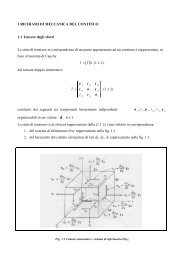
Fig. 1<br />
T-s diagram of a gas turbine engine with ITB.<br />
advantages associated with the use of ITB are an increase in thrust<br />
and potential reduction in NO x emission. 2 Recent studies on the<br />
turbine burners can be found in the literature (for example, see Liew<br />
et al., 2,3 Liu and Sirignano, 4 Sirignano and Liu, 5 and Vogeler 6 ).<br />
However, these studies are only limited to parametric cycle analysis,<br />
which is also known as on-design analysis.<br />
The work presented here is a systematic performance-cycle analysis<br />
of a dual-spool, separate-exhaust turbofan engine with an ITB.<br />
Performance-cycle analysis is also known as off-design analysis. It<br />
is an extension work for the previous study, 2,3 that is, on-design cycle<br />
analysis, in which we showed how the performance of a family<br />
of engines was determined by design choices, design limitations, or<br />
environmental conditions. 7<br />
In general, off-design analysis differs significantly from ondesign<br />
analysis. In on-design analysis, the primary purpose is to<br />
examine the variations of specific engine performance at a flight<br />
condition with changes in design parameters, including design variables<br />
for engine components. Then, it is possible to narrow the<br />
desirable range for each design parameter. Once the design choice<br />
is made, it gives a so-called reference-point (or design-point) engine<br />
for a particular application. Off-design analysis is then performed<br />
to estimate how this specific reference-point engine will behave at<br />
conditions other than those for which it was designed. Furthermore,<br />
the performance of several reference-point engines can be compared<br />
to find the most promising engine that has the best balanced<br />
performance over the entire flight envelope.<br />
Approach<br />
The station numbering for the turbofan cycle analysis with ITB<br />
is in accordance with APR 755A (Ref. 8) and is given in Fig. 2. The<br />
ITB (the transition duct) is located between stations 4.4 and 4.5.<br />
The resulting analysis gives a system of 18 nonlinear algebraic<br />
equations that are solved for 18 dependent variables. Table 1 gives<br />
the variables and constants in this analysis. As will be shown, specific<br />
values of the independent variables m and n are desirable for<br />
the computations of A 4.5 and A 8 .<br />
Off-Design Cycle Analysis<br />
The following assumptions are employed:<br />
1) The air and products of combustion behave as perfect gases.<br />
2) All component efficiencies are constant.<br />
3) The area at each engine station is constant, except the areas at<br />
stations 4.5 and 8.<br />
4) The flow is choked at the HPT entrance nozzles (station 4), at<br />
LPT entrance nozzles (station 4.5), and at the throat of the exhaust<br />
nozzles (stations 8 and 18).<br />
5) At this preliminary design phase, turbine cooling is not<br />
included.<br />
An off-design cycle analysis is used to calculate the uninstalled<br />
engine performance. The methodology is similar to those described<br />
in Mattingly 9 and Mattingly et al. 10 Two important concepts are<br />
mentioned here to help explaining the analytical method.<br />
The first is called referencing, in which the conservation of mass,<br />
momentum, and energy are applied to the one-dimensional flow of<br />
a perfect gas at an engine steady-state operating point. This leads to<br />
a relationship between the total temperatures τ and pressure ratios<br />
Independent Constant Dependent<br />
Component variable or known variable<br />
Engine M 0 , T 0 , P 0 —— ṁ 0 ,α<br />
Diffuser —— π d = f (M 0 ) ——<br />
Fan —— η f π f ,τ f<br />
Low-pressure compressor —— η cL π cL ,τ cL<br />
High-pressure compressor —— η cH π cH ,τ cH<br />
Burner T t4 π b f<br />
High-pressure turbine —— η tH , M 4 π tH ,τ tH<br />
Interstage burner T t4.5 π itb f itb<br />
Low-pressure turbine n η tL , M 4.5 , π tL ,τ tL<br />
A 4.5 = f (τ itb , n)<br />
Fan exhaust nozzle —— π fn M 18 , M 19<br />
Core exhaust nozzle m π n , M 8 , M 9<br />
A 8 = f (τ itb , m)<br />
Total number 7 —— 18<br />
Fig. 2<br />
Station numbering of a turbofan engine with ITB.<br />
π at a steady-state operating point, which can be written as f (τ, π)<br />
equal to a constant. The reference-point values (subscript R) from<br />
the on-design analysis can be used to give value to the constant<br />
and allow one to calculate the off-design parameters, as described<br />
next:<br />
f (τ, π) = f (τ R ,π R ) = constant (1)<br />
The second concept is the mass flow parameter (MFP), where the<br />
one-dimensional mass flow property per unit area can be written in<br />
the following functional form:<br />
MFP = ṁ √ T t<br />
/<br />
Pt A<br />
√<br />
= M γ g c /R{1 + [(γ − 1)/2]M 2 } (γ +1)/2(1−γ) (2)<br />
This relation is useful in calculating flow areas, or in finding any<br />
single flow quantity, provided the other four quantities are known<br />
at that station.<br />
Component Modeling<br />
In off-design analysis, there are two classes of predicting individual<br />
component performance. First, actual component characteristics<br />
can be obtained from component hardware performance data,<br />
which give a better estimate. However, in the absence of actual<br />
component hardware in a preliminary engine design phase, simple<br />
models of component performance in terms of operating conditions<br />
are used.<br />
High-Pressure Turbine<br />
Writing mass flow rate equation at stations 4 and 4.5 in terms of<br />
the flow properties and MFP gives<br />
and<br />
ṁ 4 = ( P t4<br />
/√<br />
Tt4<br />
)<br />
A4 MFP(M 4 ) =ṁ 3 (1 + f b ) (3)<br />
ṁ 4.5 = ( P t4.5<br />
/√<br />
Tt4.5<br />
)<br />
A4.5 MFP(M 4.5 ) =ṁ 3 (1 + f b + f itb ) (4)