Bayesian Methods for Regression in R - LISA
Bayesian Methods for Regression in R - LISA
Bayesian Methods for Regression in R - LISA
Create successful ePaper yourself
Turn your PDF publications into a flip-book with our unique Google optimized e-Paper software.
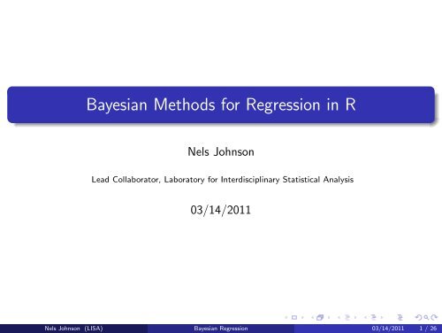
<strong>Bayesian</strong> <strong>Methods</strong> <strong>for</strong> <strong>Regression</strong> <strong>in</strong> R<br />
Nels Johnson<br />
Lead Collaborator, Laboratory <strong>for</strong> Interdiscipl<strong>in</strong>ary Statistical Analysis<br />
03/14/2011<br />
Nels Johnson (<strong>LISA</strong>) <strong>Bayesian</strong> <strong>Regression</strong> 03/14/2011 1 / 26
Outl<strong>in</strong>e<br />
What is L<strong>in</strong>ear <strong>Regression</strong>?<br />
Intro to <strong>Bayesian</strong> Statistics<br />
More on Priors<br />
<strong>Bayesian</strong> Estimation and Inference<br />
Comput<strong>in</strong>g Issues<br />
Examples<br />
Nels Johnson (<strong>LISA</strong>) <strong>Bayesian</strong> <strong>Regression</strong> 03/14/2011 2 / 26
<strong>Regression</strong><br />
Suppose you have a variable Y whose outcome is considered random.<br />
Examples: Amount of soil erosion at a particular site; How much time it<br />
takes <strong>for</strong> a fungus to develop a resistance to a fungicide; How many feet a<br />
mov<strong>in</strong>g car will need to come to a complete stop.<br />
Suppose you have some other other variables X which are treated as fixed.<br />
Examples: K<strong>in</strong>d of plants are grow<strong>in</strong>g <strong>in</strong> the soil; The composition of the<br />
fungicide; How fast the car is travel<strong>in</strong>g.<br />
If you th<strong>in</strong>k the observed value of Y is dependent on X then regression is a<br />
tool <strong>for</strong> model<strong>in</strong>g that dependence.<br />
Nels Johnson (<strong>LISA</strong>) <strong>Bayesian</strong> <strong>Regression</strong> 03/14/2011 3 / 26
L<strong>in</strong>ear <strong>Regression</strong><br />
L<strong>in</strong>ear regression assumes that the underly<strong>in</strong>g structure of Y is as l<strong>in</strong>ear<br />
comb<strong>in</strong>ation of the variables X .<br />
Example:<br />
Y dist = β 0 + X speed β speed + ɛ<br />
Often the <strong>for</strong>mula <strong>for</strong> l<strong>in</strong>ear regression will be condensed us<strong>in</strong>g matrix algebra:<br />
Y = X β + ɛ<br />
S<strong>in</strong>ce Y is considered a random variable, we will naturally expect it not to<br />
follow the underly<strong>in</strong>g structure exactly.<br />
ɛ is the term of the model that describes Y ’s random variation around it’s<br />
underly<strong>in</strong>g structure X β.<br />
The most common way to describe the random variation is with ɛ ∼ N(0, σ 2 ).<br />
Nels Johnson (<strong>LISA</strong>) <strong>Bayesian</strong> <strong>Regression</strong> 03/14/2011 4 / 26
Estimat<strong>in</strong>g Parameters<br />
S<strong>in</strong>ce we don’t know the values <strong>for</strong> β and σ 2 we’ll need to estimate them<br />
based on our data (Y , X ).<br />
Traditionally we would do so by f<strong>in</strong>d<strong>in</strong>g the β and σ 2 that maximize the<br />
likelihood:<br />
L(Y i |X i , β, σ 2 ) =<br />
n∏<br />
N(Y i |X i β, σ 2 )<br />
Note: the likelihood is also the jo<strong>in</strong>t distribution of the data.<br />
The estimates ˆβ = (X T X ) −1 X T Y and s 2 = (Y −X ˆβ) T (Y −X ˆβ)<br />
n−p<br />
would be<br />
considered random variables because they are functions of the random<br />
variable Y i .<br />
i=1<br />
Nels Johnson (<strong>LISA</strong>) <strong>Bayesian</strong> <strong>Regression</strong> 03/14/2011 5 / 26
Interpretation of Parameters<br />
We might compute a confidence <strong>in</strong>terval <strong>for</strong> β or per<strong>for</strong>m a test to see if it is<br />
significantly different from zero.<br />
Confidence <strong>in</strong>tervals are <strong>in</strong>terpreted <strong>in</strong> terms of the proportion (i.e. relative<br />
frequency) of times they should capture the true parameter <strong>in</strong> the long run.<br />
This is because it is the endpo<strong>in</strong>ts of the <strong>in</strong>terval that are random variables<br />
and the parameter is fixed. The <strong>in</strong>terval either captures the fixed parameter<br />
or it doesn’t.<br />
Because of this <strong>in</strong>terpretation, this paradigm of statistics is called the<br />
frequentist paradigm (or classical paradigm).<br />
Nels Johnson (<strong>LISA</strong>) <strong>Bayesian</strong> <strong>Regression</strong> 03/14/2011 6 / 26
Example 1.2<br />
This is an example of regression us<strong>in</strong>g the lm() function <strong>in</strong> R.<br />
Go to Example 1.2 <strong>in</strong> “Bayes Reg 2011.r”<br />
Nels Johnson (<strong>LISA</strong>) <strong>Bayesian</strong> <strong>Regression</strong> 03/14/2011 7 / 26
Bayes’ Theorem<br />
The <strong>Bayesian</strong> paradigm is named after Rev Thomas Bayes <strong>for</strong> its use of his<br />
theorem.<br />
Take the rule <strong>for</strong> conditional probability <strong>for</strong> two events A and B:<br />
P(A|B) =<br />
Bayes discovered that this is equivalent to:<br />
P(A|B) = P(B|A)P(A)<br />
P(B)<br />
P(A ∩ B)<br />
P(B)<br />
This is known as Bayes’ Theorem or Bayes’ Rule.<br />
= ∫ P(B|A)P(A)<br />
P(B|A)P(A)dA<br />
Nels Johnson (<strong>LISA</strong>) <strong>Bayesian</strong> <strong>Regression</strong> 03/14/2011 8 / 26
<strong>Bayesian</strong> Paradigm<br />
The mathematician Pierre-Simon Laplace got the idea that <strong>in</strong>stead of just<br />
def<strong>in</strong><strong>in</strong>g probability on variables, we could also def<strong>in</strong>e probability on<br />
parameters too. And by us<strong>in</strong>g Bayes’ Rule we can make <strong>in</strong>ference on<br />
parameters. Effectively treat<strong>in</strong>g parameters as random variables.<br />
In our regression example, let θ = {β, σ 2 } and D = the data. Us<strong>in</strong>g Bayes’<br />
Rule we get:<br />
P(θ|D) = P(D|θ)P(θ)<br />
P(D)<br />
P(θ|D) is called the posterior distribution. It is what we will use to make<br />
<strong>in</strong>ference about the parameters θ = {β, σ 2 }.<br />
Nels Johnson (<strong>LISA</strong>) <strong>Bayesian</strong> <strong>Regression</strong> 03/14/2011 9 / 26
<strong>Bayesian</strong> Paradigm<br />
The mathematician Pierre-Simon Laplace got the idea that <strong>in</strong>stead of just<br />
def<strong>in</strong><strong>in</strong>g probability on variables, we could also def<strong>in</strong>e probability on<br />
parameters too. And by us<strong>in</strong>g Bayes’ Rule we can make <strong>in</strong>ference on<br />
parameters. Effectively treat<strong>in</strong>g parameters as random variables.<br />
In our regression example, let θ = {β, σ 2 } and D = the data. Us<strong>in</strong>g Bayes’<br />
Rule we get:<br />
P(θ|D) = P(D|θ)P(θ)<br />
P(D)<br />
P(D|θ) is the likelihood we discussed previously. It conta<strong>in</strong>s all the<br />
<strong>in</strong><strong>for</strong>mation about θ we can learn from the data.<br />
Nels Johnson (<strong>LISA</strong>) <strong>Bayesian</strong> <strong>Regression</strong> 03/14/2011 9 / 26
<strong>Bayesian</strong> Paradigm<br />
The mathematician Pierre-Simon Laplace got the idea that <strong>in</strong>stead of just<br />
def<strong>in</strong><strong>in</strong>g probability on variables, we could also def<strong>in</strong>e probability on<br />
parameters too. And by us<strong>in</strong>g Bayes’ Rule we can make <strong>in</strong>ference on<br />
parameters. Effectively treat<strong>in</strong>g parameters as random variables.<br />
In our regression example, let θ = {β, σ 2 } and D = the data. Us<strong>in</strong>g Bayes’<br />
Rule we get:<br />
P(θ|D) = P(D|θ)P(θ)<br />
P(D)<br />
P(θ) is called the prior distribution <strong>for</strong> θ. It conta<strong>in</strong>s the <strong>in</strong><strong>for</strong>mation we<br />
know about θ be<strong>for</strong>e we observe the data.<br />
Nels Johnson (<strong>LISA</strong>) <strong>Bayesian</strong> <strong>Regression</strong> 03/14/2011 9 / 26
<strong>Bayesian</strong> Paradigm<br />
The mathematician Pierre-Simon Laplace got the idea that <strong>in</strong>stead of just<br />
def<strong>in</strong><strong>in</strong>g probability on variables, we could also def<strong>in</strong>e probability on<br />
parameters too. And by us<strong>in</strong>g Bayes’ Rule we can make <strong>in</strong>ference on<br />
parameters. Effectively treat<strong>in</strong>g parameters as random variables.<br />
In our regression example, let θ = {β, σ 2 } and D = the data. Us<strong>in</strong>g Bayes’<br />
Rule we get:<br />
P(θ|D) = P(D|θ)P(θ)<br />
P(D)<br />
P(D) is the normaliz<strong>in</strong>g constant of the function P(D|θ)P(θ) such that<br />
P(θ|D) is a proper probability distribution.<br />
Nels Johnson (<strong>LISA</strong>) <strong>Bayesian</strong> <strong>Regression</strong> 03/14/2011 9 / 26
Proportionality<br />
Often know<strong>in</strong>g the normaliz<strong>in</strong>g constant P(D) is not necessary <strong>for</strong> <strong>Bayesian</strong><br />
<strong>in</strong>ference.<br />
When it’s removed we get:<br />
P(θ|D) ∝ P(D|θ)P(θ) ⇔ posterior ∝ likelihood × prior<br />
The ∝ symbol means that P(θ|D) is proportional to (i.e. a scalar multiple<br />
of) P(D|θ)P(θ).<br />
In this case that scalar is P(D).<br />
Usually P(D|θ) and P(θ) only need to be known up to proportionality as well<br />
because their normaliz<strong>in</strong>g constants get lumped <strong>in</strong> with P(D).<br />
Nels Johnson (<strong>LISA</strong>) <strong>Bayesian</strong> <strong>Regression</strong> 03/14/2011 10 / 26
How It Works:<br />
The advantage of <strong>Bayesian</strong> analysis is sequentially updat<strong>in</strong>g beliefs about θ.<br />
Process: Prior belief about θ → Observe data → update belief about θ.<br />
That is P(θ) → P(D|θ)P(θ) → P(θ|D).<br />
Now that we’ve done one experiment and have P(θ|D 1 ) we can conduct<br />
another experiment us<strong>in</strong>g P(θ|D 1 ) as the prior <strong>for</strong> θ.<br />
Leads us to:<br />
P(θ|D 2 , D 1 ) ∝ P(D 2 |θ)P(θ|D 1 )<br />
This process can be cont<strong>in</strong>ually repeated.<br />
Example: Last year you did a study relat<strong>in</strong>g levels of heavy metals <strong>in</strong> streams<br />
to the size of mussels <strong>in</strong> the stream. Use the posterior from last year’s study<br />
as your prior <strong>for</strong> this year’s study.<br />
Nels Johnson (<strong>LISA</strong>) <strong>Bayesian</strong> <strong>Regression</strong> 03/14/2011 11 / 26
Prior Distributions<br />
Just like how you need to specify the likelihood <strong>for</strong> the problem, you need to<br />
specify the prior distribution.<br />
This is not an <strong>in</strong>tuitive process <strong>for</strong> many people at first ma<strong>in</strong>ly because of the<br />
prior.<br />
What helped me the most: th<strong>in</strong>k of the prior as a measure of our uncerta<strong>in</strong>ty<br />
<strong>in</strong> the θ’s true value.<br />
Very often it is easiest to write the jo<strong>in</strong>t prior as <strong>in</strong>dependent univariate<br />
priors, e.g. P(θ) = P(β)P(σ 2 ).<br />
Some more important term<strong>in</strong>ology that comes up when talk<strong>in</strong>g about priors:<br />
In<strong>for</strong>mative and non<strong>in</strong><strong>for</strong>mative priors<br />
Proper and improper priors<br />
Conjugate priors<br />
Reference priors<br />
Nels Johnson (<strong>LISA</strong>) <strong>Bayesian</strong> <strong>Regression</strong> 03/14/2011 12 / 26
MLE Posteriors<br />
If we use maximum likelihood to estimate β, with σ 2 known, then<br />
ˆβ = (X T X ) −1 X T Y and V ( ˆβ) = σ 2 (X T X ) −1 . We also know the sampl<strong>in</strong>g<br />
distribution <strong>for</strong> ˆβ is normal.<br />
It turns out, if we can pick the prior π(β) ∝ 1, then<br />
π(β|X , Y ) ∼ N((X T X ) −1 X T Y , σ 2 (X T X ) −1 ).<br />
This is an example improper prior, s<strong>in</strong>ce it isn’t a valid probability<br />
distribution, but the posterior π(β|X , Y ) is.<br />
It is also considered an uni<strong>for</strong>mative.<br />
In fact, it is so un<strong>in</strong><strong>for</strong>mative it’s called the reference prior, s<strong>in</strong>ce it’s the least<br />
<strong>in</strong><strong>for</strong>mative prior we could pick (under some criterion I don’t want to get<br />
<strong>in</strong>to).<br />
Nels Johnson (<strong>LISA</strong>) <strong>Bayesian</strong> <strong>Regression</strong> 03/14/2011 13 / 26
Example 1.3<br />
This example will allow us to see how the prior is updated after we see data.<br />
Key po<strong>in</strong>ts:<br />
As the sample size <strong>in</strong>creases, impact of prior on posterior decreases.<br />
As the variance of the prior <strong>in</strong>creases (i.e. diffuse prior), impact of the prior on<br />
the posterior decreases.<br />
Where the prior is centered is not important if the prior is diffuse enough.<br />
Nels Johnson (<strong>LISA</strong>) <strong>Bayesian</strong> <strong>Regression</strong> 03/14/2011 14 / 26
Conjugacy<br />
If P(θ) is a conjugate prior <strong>for</strong> θ with likelihood P(D|θ), then P(θ|D) has the<br />
same family of distributions as the prior.<br />
This is nice because it means that <strong>in</strong> some cases we can pick a prior such<br />
that the posterior distribution will be a distribution we understand well (e.g.<br />
normal, gamma).<br />
This means computational methods might not be needed <strong>for</strong> <strong>in</strong>ference or that<br />
the computation methods will be fast and simple to implement.<br />
For a list of some: http://en.wikipedia.org/wiki/Conjugate_prior<br />
Nels Johnson (<strong>LISA</strong>) <strong>Bayesian</strong> <strong>Regression</strong> 03/14/2011 15 / 26
Common Conjugate Examples<br />
Y = X β + ɛ where ɛ ∼ N(0, σ 2 I ) or ɛ ∼ N(0, Σ)<br />
Parameter Prior Likelihood Posterior<br />
β Normal Normal Normal<br />
σ 2 Inverse-Gamma Normal Inverse-Gamma<br />
Σ Inverse-Wishart Normal Inverse-Wishart<br />
σ −2 Gamma Normal Gamma<br />
Σ −1 Wishart Normal Wishart<br />
Nels Johnson (<strong>LISA</strong>) <strong>Bayesian</strong> <strong>Regression</strong> 03/14/2011 16 / 26
To R<br />
The rest of this presentation will be <strong>in</strong> R.<br />
I’ve left all my slides from an older version of this talk <strong>for</strong> those that may be<br />
<strong>in</strong>terested <strong>in</strong> read<strong>in</strong>g them later.<br />
Nels Johnson (<strong>LISA</strong>) <strong>Bayesian</strong> <strong>Regression</strong> 03/14/2011 17 / 26
Posterior Distributions<br />
<strong>Bayesian</strong> <strong>in</strong>ference is usually done on the jo<strong>in</strong>t posterior distribution of all the<br />
parameters P(θ|D).<br />
Sometimes it is done on the marg<strong>in</strong>al distribution of a s<strong>in</strong>gle parameter. Such<br />
as:<br />
∫<br />
P(β|D) = P(θ|D)dσ 2<br />
Because the posterior is a probability distribution <strong>for</strong> θ, pre<strong>for</strong>m<strong>in</strong>g <strong>in</strong>ference<br />
on θ is as simple as f<strong>in</strong>d<strong>in</strong>g relevant summaries based on its posterior.<br />
Nels Johnson (<strong>LISA</strong>) <strong>Bayesian</strong> <strong>Regression</strong> 03/14/2011 18 / 26
Po<strong>in</strong>t Estimation<br />
Two very popular po<strong>in</strong>t estimators <strong>for</strong> θ:<br />
The mean of the posterior distribution (posterior mean).<br />
The maximum a posterior estimator also known as the MAP estimator.<br />
The MAP estimator is arg max θ P(θ|D).<br />
You could use any measure of center that makes sense <strong>for</strong> P(θ|D).<br />
Nels Johnson (<strong>LISA</strong>) <strong>Bayesian</strong> <strong>Regression</strong> 03/14/2011 19 / 26
Illustration of MAP Estimator<br />
Nels Johnson (<strong>LISA</strong>) <strong>Bayesian</strong> <strong>Regression</strong> 03/14/2011 20 / 26
Interval Estimation<br />
<strong>Bayesian</strong> confidence <strong>in</strong>tervals are called credible <strong>in</strong>tervals. So a 95% <strong>Bayesian</strong><br />
confidence <strong>in</strong>terval is called a 95% credible <strong>in</strong>terval.<br />
There are two popular ways to f<strong>in</strong>d them:<br />
Highest posterior density, often shortened to HPD.<br />
Equal tail probability.<br />
A 95% HPD credible <strong>in</strong>terval is the smallest <strong>in</strong>terval with probability 0.95.<br />
A 95% Equal tail probability <strong>in</strong>terval use the values that have cumulative<br />
probability of 0.025 and 0.975 as the endpo<strong>in</strong>ts. This is not preferred when<br />
the posterior is highly skewed or multimodal.<br />
Nels Johnson (<strong>LISA</strong>) <strong>Bayesian</strong> <strong>Regression</strong> 03/14/2011 21 / 26
HPD and Equal Tail Credible Intervals<br />
Nels Johnson (<strong>LISA</strong>) <strong>Bayesian</strong> <strong>Regression</strong> 03/14/2011 22 / 26
Hypothesis Test<strong>in</strong>g<br />
S<strong>in</strong>ce we can talk about the probability of θ be<strong>in</strong>g <strong>in</strong> some <strong>in</strong>terval, this make<br />
<strong>in</strong>terpretation of certa<strong>in</strong> k<strong>in</strong>ds of hypothesis tests much easier.<br />
For <strong>in</strong>stance H 0 : β ≤ 0 vs. H a : β ≥ 0 You can f<strong>in</strong>d P β|D (β ≤ 0) and if it is<br />
sufficiently small then reject the null hypothesis <strong>in</strong> favor of the alternative.<br />
We could also test H 0 : a ≤ β ≤ b vs H 0 : β ≤ a or b ≤ β where a and b are<br />
chosen such that if H 0 were true them then β would have no practical effect.<br />
Aga<strong>in</strong>, compute P β|D (H 0 ) and if it is sufficiently small, reject H 0 .<br />
Some special steps need to be take when try<strong>in</strong>g to test H 0 : β = 0 which are<br />
beyond the scope of this course.<br />
Also <strong>in</strong>stead of reject<strong>in</strong>g H 0 or accept<strong>in</strong>g H a , you could just report the<br />
evidence (i.e. the probability) <strong>for</strong> the reader to decide.<br />
Nels Johnson (<strong>LISA</strong>) <strong>Bayesian</strong> <strong>Regression</strong> 03/14/2011 23 / 26
Sampl<strong>in</strong>g From the Jo<strong>in</strong>t Posterior<br />
As stated previously we want to per<strong>for</strong>m <strong>in</strong>ference on θ us<strong>in</strong>g the jo<strong>in</strong>t<br />
posterior P(θ|D).<br />
Summariz<strong>in</strong>g the jo<strong>in</strong>t posterior may be difficult (or impossible).<br />
A solution to this problem is to use a computer algorithm to sample<br />
observations from the jo<strong>in</strong>t posterior.<br />
If we have a large enough sample from P(θ|D) then the distribution of the<br />
sample should approximate P(θ|D).<br />
This means we can just summarize the sample from P(θ|D) to make<br />
<strong>in</strong>ference on θ <strong>in</strong>stead of us<strong>in</strong>g the distribution P(θ|D) directly.<br />
Nels Johnson (<strong>LISA</strong>) <strong>Bayesian</strong> <strong>Regression</strong> 03/14/2011 24 / 26
One (Three) Important Algorithm(s)<br />
The big three algorithms are as follows:<br />
Gibbs sampl<strong>in</strong>g.<br />
Metropolis algorithm.<br />
Metropolis-Hast<strong>in</strong>gs algorithm.<br />
All three of these algorithms are Markov Cha<strong>in</strong> Monte Carlo algorithms.<br />
Commonly known as MCMC algorithms.<br />
What that means <strong>for</strong> us is that after you run the algorithm “long enough”<br />
you will eventually start sampl<strong>in</strong>g from P(θ|D).<br />
The Metropolis-Hast<strong>in</strong>g algorithm is a generalization of the other two and it<br />
so similar to the Metropolis algorithm that the two titles are often<br />
<strong>in</strong>terchanged.<br />
Nels Johnson (<strong>LISA</strong>) <strong>Bayesian</strong> <strong>Regression</strong> 03/14/2011 25 / 26
More on Gibbs<br />
The Gibbs sampler is a much simplified version of the Metropolis-Hast<strong>in</strong>gs<br />
algorithm. So simplified <strong>in</strong> fact it isn’t obvious at all that they are related.<br />
All three algorithms require you to know the conditional posterior distribution<br />
of each parameter <strong>in</strong> the model (e.g. P(β|D, σ 2 ) and P(σ 2 |D, β) ).<br />
The Gibbs sampler requires that the user can sample from each of the<br />
conditional posterior distributions us<strong>in</strong>g computer software.<br />
This is where conjugate priors become very popular. If the conditional<br />
posterior distributions are all normal, gamma, or some other distribution we<br />
can readily sample from, then the Gibbs algorithm makes sampl<strong>in</strong>g from the<br />
jo<strong>in</strong>t posterior very easy.<br />
Other details about this algorithm are beyond the scope of this course.<br />
The data analysis examples we will discuss both use a Gibbs sampler.<br />
Nels Johnson (<strong>LISA</strong>) <strong>Bayesian</strong> <strong>Regression</strong> 03/14/2011 26 / 26


