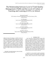
evaluation and performance analysis of propagation models for wimax

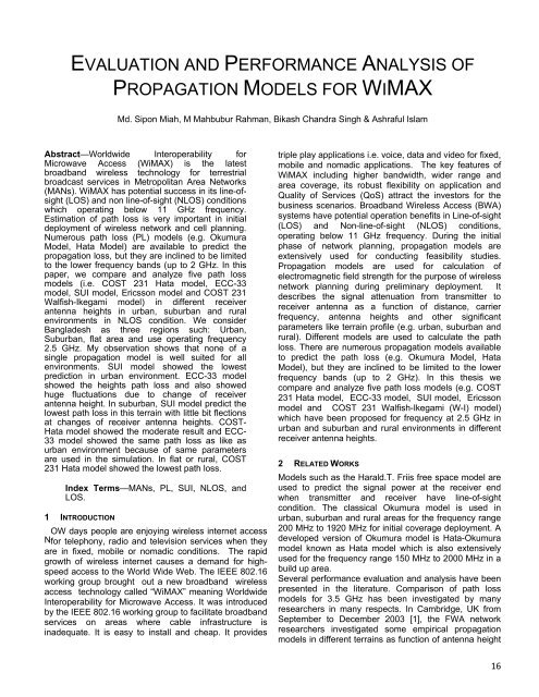
EVALUATION AND PERFORMANCE ANALYSIS OFPROPAGATION MODELS FOR WIMAXMd. Sipon Miah, M Mahbubur Rahman, Bikash Chandra Singh & Ashraful IslamAbstract—Worldwide Interoperability forMicrowave Access (WiMAX) is the latestbroadband wireless technology for terrestrialbroadcast services in Metropolitan Area Networks(MANs). WiMAX has potential success in its line-ofsight(LOS) and non line-of-sight (NLOS) conditionswhich operating below 11 GHz frequency.Estimation of path loss is very important in initialdeployment of wireless network and cell planning.Numerous path loss (PL) models (e.g. OkumuraModel, Hata Model) are available to predict thepropagation loss, but they are inclined to be limitedto the lower frequency bands (up to 2 GHz. In thispaper, we compare and analyze five path lossmodels (i.e. COST 231 Hata model, ECC-33model, SUI model, Ericsson model and COST 231Walfish-Ikegami model) in different receiverantenna heights in urban, suburban and ruralenvironments in NLOS condition. We considerBangladesh as three regions such: Urban,Suburban, flat area and use operating frequency2.5 GHz. My observation shows that none of asingle propagation model is well suited for allenvironments. SUI model showed the lowestprediction in urban environment. ECC-33 modelshowed the heights path loss and also showedhuge fluctuations due to change of receiverantenna height. In suburban, SUI model predict thelowest path loss in this terrain with little bit flectionsat changes of receiver antenna heights. COST-Hata model showed the moderate result and ECC-33 model showed the same path loss as like asurban environment because of same parametersare used in the simulation. In flat or rural, COST231 Hata model showed the lowest path loss.Index Terms—MANs, PL, SUI, NLOS, andLOS.1 INTRODUCTIONOW days people are enjoying wireless internet accessN for telephony, radio and television services when theyare in fixed, mobile or nomadic conditions. The rapidgrowth of wireless internet causes a demand for highspeedaccess to the World Wide Web. The IEEE 802.16working group brought out a new broadband wirelessaccess technology called “WiMAX” meaning WorldwideInteroperability for Microwave Access. It was introducedby the IEEE 802.16 working group to facilitate broadbandservices on areas where cable infrastructure isinadequate. It is easy to install and cheap. It providestriple play applications i.e. voice, data and video for fixed,mobile and nomadic applications. The key features ofWiMAX including higher bandwidth, wider range andarea coverage, its robust flexibility on application andQuality of Services (QoS) attract the investors for thebusiness scenarios. Broadband Wireless Access (BWA)systems have potential operation benefits in Line-of-sight(LOS) and Non-line-of-sight (NLOS) conditions,operating below 11 GHz frequency. During the initialphase of network planning, propagation models areextensively used for conducting feasibility studies.Propagation models are used for calculation ofelectromagnetic field strength for the purpose of wirelessnetwork planning during preliminary deployment. Itdescribes the signal attenuation from transmitter toreceiver antenna as a function of distance, carrierfrequency, antenna heights and other significantparameters like terrain profile (e.g. urban, suburban andrural). Different models are used to calculate the pathloss. There are numerous propagation models availableto predict the path loss (e.g. Okumura Model, HataModel), but they are inclined to be limited to the lowerfrequency bands (up to 2 GHz). In this thesis wecompare and analyze five path loss models (e.g. COST231 Hata model, ECC-33 model, SUI model, Ericssonmodel and COST 231 Walfish-Ikegami (W-I) model)which have been proposed for frequency at 2.5 GHz inurban and suburban and rural environments in differentreceiver antenna heights.2 RELATED WORKSModels such as the Harald.T. Friis free space model areused to predict the signal power at the receiver endwhen transmitter and receiver have line-of-sightcondition. The classical Okumura model is used inurban, suburban and rural areas for the frequency range200 MHz to 1920 MHz for initial coverage deployment. Adeveloped version of Okumura model is Hata-Okumuramodel known as Hata model which is also extensivelyused for the frequency range 150 MHz to 2000 MHz in abuild up area.Several performance evaluation and analysis have beenpresented in the literature. Comparison of path lossmodels for 3.5 GHz has been investigated by manyresearchers in many respects. In Cambridge, UK fromSeptember to December 2003 [1], the FWA networkresearchers investigated some empirical propagationmodels in different terrains as function of antenna height16

The Hata model is introduced as a mathematicalexpression to mitigate the best fit of the graphical dataprovided by the classical Okumura model. Hata model isused for the frequency range of 150 MHz to 1500 MHz topredict the median path loss for the distance d fromtransmitter to receiver antenna up to 20 km, andtransmitter antenna height is considered 30 m to 200 mand receiver antenna height is 1 m to 10 m. To predictthe path loss in the frequency range 1500 MHz to 2000MHz. COST 231 Hata model is initiated as an extensionof Hata model. The basic path loss equation for thisCOST-231 Hata Model can be expressed as:PL = 46.3 + 33.9 log 10 (f) – 13.82 log 10 (h b ) – ah m + (44.9– 6.55 log 10 (h b )) log 10 d + c m6whered : Distance between transmitter and receiver antenna[km]f : Frequency [MHz]h b : Transmitter antenna height [m]The parameter c m has different values for differentenvironments like 0 dB for suburban and 3 dB for urbanareas and the remaining parameter ah m is defined inurban areas as:ah m = 3.20(log 10 (11.75h r )) 2 – 4.79 for f > 400 MHz7The value for ah m in suburban and rural (flat) areas isgiven as:IRACST - International Journal of Advanced Computing, Engineering and Application (IJACEA),Vol. 1, No.1, 2012: Wavelength [m]: Correction for frequency above 2 GHz [MHz]: Correction for receiving antenna height [m]: Correction for shadowing [dB]: Path loss exponentThe random variables are taken through a statisticalprocedure as the path loss exponent γ and the weakfading standard deviation s is defined. The log normallydistributed factor s, for shadow fading because of treesand other clutter on a propagations path and its value isbetween 8.2 dB and 10.6 dB. The parameter A is definedasAnd the path loss exponent γ is given by10+ 11Where, the parameter h b is the base station antennaheight in meters. This is between 10 m and 80 m. Theconstants a, b, and c depend upon the types of terrain,that are given in Table 3. The value of parameter γ = 2for free space propagation in an urban area, 3 < γ < 5 forurban NLOS environment, and γ > 5 for indoorpropagation.The frequency correction factor and the correction forreceiver antenna height for the model are expressedinah m = (1.11log 10 f – 0.7)h r – (1.5 log 10 f – 0.8)8Where theis the receiver antenna height in meter.4.5 Stanford University Interim (SUI) ModelIEEE 802.16 Broadband Wireless Access working groupproposed the standards for the frequency band below 11GHz containing the channel model developed byStanford University, namely the SUI models. Thisprediction model comes from the extension of Hatamodel with frequency larger than 1900 MHz. Thecorrection parameters are allowed to extend this modelup to 2.5 GHz band. The base station antenna height ofSUI model can be used from 10 m to 80 m. Receiverantenna height is from 2 m to 10 m. The cell radius isfrom 0.1 km to 8 km. The basic path loss expression ofThe SUI model with correction factors is presented as:ForWhere the parameters are: Distance between BS and receiving antenna [m]: 100 [m]9Where, f is the operating frequency in MHz, and h r is thereceiver antenna height in meter. For the abovecorrection factors this model is extensively used for thepath loss prediction of all three types of terrain in rural,urban and suburban environments.4.6 Hata-Okumura Extended Model or ECC-33 ModelThe original Okumura model doesn’t provide any datagreater than 3 GHz. Based on prior knowledge ofOkumura model; an extrapolated method is applied topredict the model for higher frequency greater than 3GHz. The tentatively proposed propagation model ofHata-Okumura model with report is referred to as ECC-33 model. In this model path loss is given by14: Free space attenuation [dB]: Basic median path loss [dB]: Transmitter antenna height gain factor121319

: Receiver antenna height gain factorThese factors can be separately described and given byas=92.4+20 15=20.41+9.83log 10 (d) + 20 log 10 (f) + 9.56Where23[log 10 (f)] 2 16 1616= 17When dealing with gain for medium cities, the will beexpressed in=For large city18= 19Where: Distance between transmitter and receiverAntenna [km]: Frequency [GHz]: Transmitter antenna height [m]: Receiver antenna height [m]This model is the hierarchy of Okumura-Hata model.4.8 COST 231 Walfish-Ikegami (W-I) ModelThis model is a combination of J. Walfish and F. Ikegamimodel. This model is most suitable for flat suburban andurban areas that have uniform building height. Theequation of the proposed model is expressed in:For LOS condition16Note thatThe multi-screen diffraction loss isWhere242526And for NLOS conditionFor urban and suburbanIf L rst + L msd >0Where= Free space loss= Roof top to street diffraction= Multi-screen diffraction lossFree space loss2021272829= 22Roof top to street diffractionfor suburban of medium size cities with moderate treedensity fot metropolitan / urban.where: Distance between transmitter and receiverantenna [m]: Frequency [GHz]: Building to building distance [m]: Street width [m]20

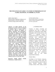
: Street orientation angel w.r.t. direct radio path[degree]In our simulation we use the following data, i.e.building to building distance 50 m, street width 25 m,street orientation angel 30 degree in urban area and 40degree in suburban area and average building height 15m, base station height 30 m.4.9 Ericsson ModelTo predict the path loss, the network planningengineers are used software provided by EricssonCompany is called Ericsson model. This model alsostands on the modified Okumura-Hata model to allowroom for changing in parameters according to thepropagation environment. Path loss according to thismodel is given by30Whereis defined byIRACST - International Journal of Advanced Computing, Engineering and Application (IJACEA),Vol. 1, No.1, 2012Fig. 1. Simulationfor three differentprocess flow chartenvironments.In this model I have used three different environments(Urban, Suburban and Flat) with different parameter.5.3 Simulation ParameterThe following Table 4.2 presents the parameters weapplied in our simulation.ParametersValuesTransmitterheightantennaReceiver antenna heightOperating frequencyEND40 m in urban and 30m in suburban and20 m in rural area3 m, 6 m and 10 m2.5 GHzAnd parameters: Frequency [MHz]: Transmission antenna height [m]: Receiver antenna height [m]31Distance between Tx-RxBuilding to buildingdistanceAverage building heightStreet width5 km50 m15 m25 m5 SIMULATION ENVIRONMENT & MODELS5.1 Simulation EnvironmentFor analyzing the performance of propagation models forWiMAX, I have used MATLAB software package.MATLAB is a software package for high-performancenumerical computation and visualization. It provides aninteractive environment with hundred of built-in functionfor technical computation, graphics and animation. Bestof all, it also provides easy extensibility with its own highprogramminglanguage. The name MATLAB stands forMATrix LABoratory.5.2 Simulation DesignFor evaluating and analyzing the performance ofWiMAX propagation models I have used MATLABsimulation. A typical simulation model is shown in fig(4.1).Street orientation angle 30 0 in urban and 40 0in suburbanCorrection for shadowing 8.2 dB in suburban andrural and10.6 dB in urban areaTable 4.1: Simulation parameters6 PERFORMANCE ANALYSIS & DISCUSSION6.1 Analysis of simulation results in urban areaIn our calculation, we set 3 different antenna heights (i.e.3 m, 6 m and 10 m) for receiver, distance varies from250 m to 5 km and transmitter antenna height is 40 m.The numerical results for different models in urban areafor different receiver antenna heights are shown in theFigure 2, 3 and 4.STARTInput ParameterChooseEnvironmentOutput Path lossFig. 2. Path loss in urban environment at 3 m receiverantenna height.21

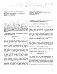
UrbanP a t h l o s s d B20015010050156154150 154150147138136135126124121149147142109 109 1090ECC-33 COST-Hata ERICSSON SUI COST-WI FSPLFig. 3. Path loss in urban environment at 6 m receiverantenna height.Rx height 3m 156 154 138 126 149 109Rx height 6m 154 150 136 124 147 109Rx height 10m 150 147 135 121 142 109Distance at 2.5 kmFig. 5. Analysis of simulation results for urbanenvironment in different receiver antenna height.6.2 Analysis of simulation results in Suburban areaIn our calculation, we set 3 different antenna heights (i.e.3 m, 6 m and 10 m) for receiver, distance varies from250 m to 5 km and transmitter antenna height is 30 m.The numerical results for different models in urban areafor different receiver antenna heights are shown in theFigure 6, 7 and 8.Fig.4. Path loss in urban environment at 10 m receiverantenna height.The accumulated results for urban environment areshown in figure 5. Note that SUI model showed thelowest prediction (128 dB to 121 dB) in urbanenvironment. It also showed the lowest fluctuationscompare to other models when we changed the receiverantenna heights. In that case, the ECC-33 modelshowed the heights path loss (156 dB) and also showedhuge fluctuations due to change of receiver antennaheight. In this model, path loss is decreased whenincreased the receiver antenna height. Increase thereceiver antenna heights will provide the more probabilityto find the better quality signal from the transmitter. ECC-33 model showed the biggest path loss at 10 m receiverantenna height.Fig. 6. Path loss in suburban environmentat 3 m receiver antenna height22

IRACST - International Journal of Advanced Computing, Engineering and Application (IJACEA),Vol. 1, No.1, 2012RuralPath loss dB20015010050154144154152150148143132137121 121 121109 109 109 109 109 1090COST-Hata ERICSSON SUI COST-WI FSPL FSPLRx height 3m 154 154 148 121 109 109Rx height 6m 144 152 143 121 109 109Rx height 10m 132 150 137 121 109 109Distance at 2.5 kmFig. 7. Path loss in suburban environment at 6 mreceiver antenna height.Fig. 9. Analysis of simulation results for suburbanenvironment in different receiver antenna height.6.3 Analysis of simulation results in flat areaWe set 3 different antenna heights (i.e. 3 m, 6 m and 10m) for receiver, distance varies from 250 m to 5 km andtransmitter antenna height is 20 m. COST 231 W-I modelhas no specific parameters for rural area, we considerLOS equation provided by this model The numericalresults for different models in urban area for differentreceiver antenna heights are shown in the Figure 10, 11,and 12.Fig. 8. Path loss in suburban environment at 10 mreceiver antenna height.The accumulated results for suburban environment areshown in figure 9. In following chart, it showed that theSUI model predict the lowest path loss (121 dB to 116dB) in this terrain with little bit flections at changes ofreceiver antenna heights. Ericsson model showed theheights path loss (160 dB and 158 dB) predictionespecially at 6 m and 10 m receiver antenna height. TheCOST-WI model showed the moderate result withremarkable fluctuations of path loss with-respect-toantenna heights changes. The ECC-33 model showedthe same path loss as like as urban environmentbecause of same parameters are used in the simulation.Fig. 10. Path loss in rural environment at 3 m receiverantenna height.23

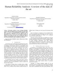
Fig. 13. Analysis of simulation results for ruralenvironment in different receiver antenna height.Fig. 11. Path loss in rural environment at 6 m receiverantenna height.Fig. 12. Path loss in rural environment at 10 m receiverantenna height.The accumulated results for rural environment are shownin Figure 13. In this environment COST 231 Hata modelshowed the lowest path loss (132 dB) predictionespecially in 10 m receiver antenna height. COST 231W-I model showed the flat results in all changes ofreceiver antenna heights. There are no specificparameters for rural area. In our simulation, weconsidered LOS equation for this environment (thereason is we can expect line of sight signal if the area isflat enough with less vegetations). Ericsson modelshowed the heights path loss (154 dB to 150 dB).Path loss dB200150100500Rural154144154152150148143132137121 121 121Distance at 2.5 km109 109 109 109 109 109COST-Hata ERICSSON SUI COST-WI FSPL FSPLRx height 3m 154 154 148 121 109 109Rx height 6m 144 152 143 121 109 109Rx height 10m 132 150 137 121 109 1097 CONCLUSIONOur comparative analysis indicate that due to multipathand NLOS environment in urban and suburban area, SUImodels experiences lowest path losses compare to flatarea. In flat area COST-Hata model provide lowest pathloss than SUI model at 10 m receiver antenna height.Moreover, we did not find any single model that can berecommended for all environments.We can see in urban area (data shown in Figure 5), theSUI model showed the lowest path loss (121 dB in 10 mreceiver antenna height) as compared to other models.Alternatively, the ECC-33 model showed the heightspath loss (156 dB in 3 m receiver antenna height).In suburban area (data shown in Figure 9) the SUI modelshowed quite less path loss (116 dB) compared to othermodels. On the other hand, ECC-33 model showedheights path loss as showed in urban area. Moreover,Ericsson model showed remarkable higher path loss for6 m and 10 m receiver antenna heights (i.e.160 dB and158 dB respectively).In rural area (data shown in Figure 13), we can choosedifferent models for different perspectives. If the area isflat enough with less vegetation, where the LOS signalprobability is high, in that case, we may consider LOScalculation. Alternatively, if there is less probability to getLOS signal, in that situation, we can see COST-Hatamodel showed the less path loss (132 dB) compare toSUI model (137 dB) and Ericsson model (150 dB)especially in 10 m receiver antenna height. Butconsidering all receiver antenna heights SUI modelshowed less path loss (148 dB in 3 m and 143 dB in 6 m)whereas COST-Hata showed higher path loss (154 dB in3m and 144 dB in 6 m).If we consider the worst case scenario for deploying acoverage area, we can serve the maximum coverage byusing more transmission power, but it will increase theprobability of interference with the adjacent area with thesame frequency blocks. On the other hand, if weconsider less path loss model for deploying a cellularregion, it may be inadequate to serve the wholecoverage area. Some users may be out of signal in theoperating cell especially during mobile condition. So, wehave to trade-off between transmission power andadjacent frequency blocks interference while choosing apath loss model for initial deployment.8 FUTURE WORKSThis is a formal ending of very small stage of a neverending process. Nowadays the WorldwideInteroperability of Microwave Access (WiMAX)technology becomes popular and receives growingacceptance as a Broadband Wireless Access (BWA)system. In future, our simulated results can be testedand verified in practical field. We may also derive a24

suitable path loss model for all terrain. Future study canbe made for finding more suitable parameters forEricsson and COST 231 W-I models in rural area.REFERENCES:[1] V.S. Abhayawardhana, I.J. Wassel, D. Crosby, M.P.Sellers, M.G. Brown, “Comparison of empiricalpropagation path loss models for fixed wirelessaccess systems,” 61th IEEE TechnologyConference, Stockholm, pp. 73-77, 2005.[2] Josip Milanovic, Rimac-Drlje S, Bejuk K,“Comparison of propagation model accuracy forWiMAX on 3.5GHz,” 14th IEEE Internationalconference on electronic circuits and systems,Morocco, pp. 111-114. 2007.[3] Joseph Wout, Martens Luc, “Performance evaluationof broadband fixed wireless system based on IEEE802.16,” IEEE wireless communications andnetworking Conference, Las Vegas, NV, v2, pp.978-983, April 2006.[4] M. Hata, “Empirical formula for propagation loss inland mobile radio services,” IEEE Transactions onVehicular Technology, vol. VT-29, pp. 317-325,September 1981.[5] Sara Abelession “Propagation measurement at 3.5GHz for WiMAX” March 2007.[6] Cem Akkaşlı, “Methods for Path loss Prediction”October 2009.[7] Propagation models for wireless mobilecommunications D. Vanhoenacker-Janvier,Microwave Lab. UCL, Louvain-la-Neuve,Belgium.[8] T.S Rappaport, Wireless Communications:Principles and Practice, 2n Ed. New delhi: PrenticeHall, 2005 pp. 151-152.[9] Well known propagation model, [Online]. Available:http://en.wikipedia.org/wiki/Radio_propagation_model [Accessed: April 11, 2009][10] IEEE 802.16 working group, [Online]. Available:http://en.wikipedia.org/wiki/IEEE_802.16 [Accessed:April 11, 2009][11] Jeffrey G Andrews, Arunabha Ghosh, RiasMuhamed, “Fundamentals of WiMAX: understandingBroadband Wireless Networking”, Prentice Hall,2007[12] WiMAX Forum, “Documentation, TechnologyWhitepapers”, [Online]. Available at WiMAXForum.org:http://www.wimaxforum.org/resources/documents[Accessed: April 18, 2008[13] Doppler spread, [Online]. Available:http://en.wikipedia.org/wiki/Fading [Accessed: April11, 2009][14] Electronic Communication Committee (ECC) withinthe European Conference of Postal andTelecommunication Administration (CEPT), “TheIRACST - International Journal of Advanced Computing, Engineering and Application (IJACEA),Vol. 1, No.1, 2012analysis of the coexistence of FWA cells in the 3.4 –3.8 GHz band,” tech. rep., ECC Report 33, May2003.[15] Rony Kowalski, “The Benefits of Dynamic AdaptiveModulation for High Capacity Wireless BackhaulSolutions”, Ceragon Networks, [Online]. Available:http://www.ceragon.com/files/The%20Benefits%20of%20Dynamic%20Adaptive%20Modulation.pdf[Accessed: April 18, 2009].[16] D. Pareek, The Business of WiMAX, Chapter 2 andChapter 4, John Wiley, 2006[17] Empirical Models, [Online] Available:http://en.wikipedia.org/wiki/Empirical_model[Accessed April 18, 2009][18] Simic I. lgor, Stanic I., and Zrnic B., “Minimax LSAlgorithm for Automatic Propagation Model Tuning,”Proceeding of the 9th Telecommunications Forum(TELFOR 2001), Belgrade, Nov.2001[19] Federal Communications Commission, “What isBroadband”, [Online]. Availablehttp://www.fcc.gov/cgb/broadband.html [Accessed:Nov 13, 2008][20] Kabelfri og mobil IT-systemanvendelse, “802.11Standard”, [Online]. Available:http://wlan.nat.sdu.dk/802_11standard.htm[Accessed: Nov 27, 2008][21] WiMAX.com, “WiMAX Reference Architecture”,[Online].Available:http://www.wimax.com/commentary/wimax_weekly/2-6-reference-network-architecturecontin[Accessed: Dec 02, 2008][22] LigatureSoft, “Data Transmission Impairments”,[Online].Available:http://www.ligaturesoft.com/data_communications/trans-impairment.html [Accessed:Dec 06,2008]Md. Sipon Miah received the Bachelor’s and Master‘sDegree in the Department of Information andCommunication Engineering from Islamic University,Kushtia, in 2006 and 2007, respectively. He is courrentlyLecturer in the department of ICE, Islamic University,Kushtia-7003, Bangladesh. Since 2003, he has been aResearch Scientist at the Communication ResearchLaboratory, Department of ICE, Islamic University,Kushtia, where he belongs to the spread-spectrumresearch group. He is pursuing research in the area ofinternetworking in wireless communication. He has tenpublished paper in international and two nationaljournals in the same areas. His areas of interest. Includedatabase system, optical fiber communication, SpreadSpectrum and mobile communication.M. Mahbubur Rahman received the Bachelor’s andMaster‘s Degree in Physics, Rajshahi University, in 1983,1994 and PhD degree in Computer Science &Engineering in 1997. He is courrently Professor in thedepartment of ICE, Islamic University, Kushtia-7003,Bangladesh. He has twenty four published papers ininternational and national journals. His areas of interestinclude internetworking, AI & mobile communication.Bikash Chandran Singh received the Bachelor’s and25

Master‘s Degree in Information and CommunicationEngineering from Islamic University, Kushtia, in 2005 and2007, respectively. He is courrently Lecturer in thedepartment of ICE, Islamic University, Kushtia-7003,Bangladesh. His areas of interest including database,optical fiber communication & multimedia.Ashraful Islam received the Bachelor’s Degree andM.SC in Information and Communication Engineeringfrom Islamic University, Kushtia, in 2008 and 2009respectively. He was completed M.Sc student in thedepartment of ICE, Islamic University, Kushtia-7003,Bangladesh. He is currently Assistant Programmer inBangladesh Computer Council, Dhaka.26