FEEDBACK CONTROL SYSTEMS

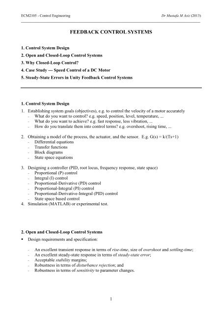
ECM2105 - Control Engineering Dr Mustafa M Aziz (2013)________________________________________________________________________________Open-loop control system: utilises an actuating device to control the process (plant) directlywithout using feedback.InputActuatingdeviceProcess orplantOutputClosed-loop control system: uses a measurement of the output and feedback of this signal tocompare it with the desired input (reference or command).R(s)E(s)U(s)G c(s)+ _G(s)Y(s)H(s)Notation:R(s): Laplace transform of the input signal;U(s): Laplace transform of the control or actuating signal;Y(s): Laplace transform of the output signal;E(s): Laplace transform of the error signal;G c (s): Transfer function of the controller;G(s): Transfer function of the process or plant;H(s): Transfer function of the sensor.2

ECM2105 - Control Engineering Dr Mustafa M Aziz (2013)________________________________________________________________________________3. Why Closed-Loop Control?An advantage of the closed-loop control system is the fact that the use of feedback makes thesystem response relatively insensitive to external disturbances (e.g. temperature and pressure) andinternal variations in system parameters (e.g. component tolerances) which are not known orpredicted.3.1. Sensitivity of control systems to parameter variationsSuppose that G(s) changes to G(s)+∆G(s) due to the environment, ageing, etc. For small ∆G(s)

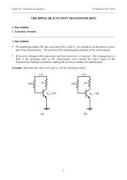
ECM2105 - Control Engineering Dr Mustafa M Aziz (2013)________________________________________________________________________________3.2. Disturbance rejectionSuppose that there is an input disturbance D(s) applied between the controller and plant:D(s)Open-loop:U(s) = G c (s)R(s)Y(s) = G c (s)G(s)R(s)+G(s)D(s)R(s)G c(s)+U(s) +G(s)Y(s)Closed-loop: U(s) = G c (s)[R(s) – H(s)Y(s)]Gc(s)G(s)Y(s) =R(s)1+G (s)G(s)H(s)cG(s)+D(s)1+G (s)G(s)H(s)cR(s)D(s)+U(s) +G c(s)+ –H(s)G(s)Y(s)Exercise: For the systems shown above, the process transfer function G(s) = 1/(0.5s+1), thecontroller G c (s) = 99, R = 0, a step-unit disturbance D(s) = 1/s, and H(s) = 1. Determine theresponse to the disturbance for both the open-loop and closed-loop systems and sketch the outputs.4

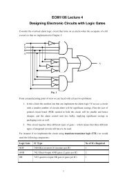
ECM2105 - Control Engineering Dr Mustafa M Aziz (2013)________________________________________________________________________________3.3. Transient responseThe transient response is the response of a system as a function of time.A motor speed control system:− Objective: the actual speed y approaches the desired speed r quickly− Open-loop: G c (s) = k, G(s) = k 1 /(Ts+1)Assume, for example, kk 1 = 1, T = 10− Closed-loop with a proportional control term k, H(s) = 1Assume, for example, kk 1 = 10, T = 10.1Unit-step response of open-loop control1Unit-step response of closed-loop control0.90.90.80.80.70.7Amplitude0.60.50.4Amplitude0.60.50.40.30.30.20.20.10.100 5 10 15Time (sec.)00 5 10 15Time (sec.)3.4. Steady-state errorThe steady-state error is the error after the transient response has decayed, leaving only thecontinuous response, that is for a unity-feedback system:e( ∞)= lim[r(t) − y(t)]t→∞E(s) = R(s) - Y(s). Considering a unit-step input, R(s) = 1/s:− Open-loop: Y(s) = G(s)R(s), E(s) = [1-G(s)]R(s).By the final-value theorem,e( ∞)= lime(t) = limsE(s) = 1−G(0)t→∞− Closed-loop: Y(s) = G(s)R(s)/[1+G(s)H(s)]. For H(s) = 1, E(s) = R(s)/[1+G(s)]By the final-value theorem,s→0e( ∞)= lime(t) = limsE(s) = 1/[1 + G(0)]t→∞s→05

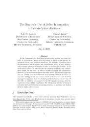
ECM2105 - Control Engineering Dr Mustafa M Aziz (2013)________________________________________________________________________________4. Case Study --- Speed Control of a DC MotorThe purpose of this case study is: to compare the open-loop and closed-loop control, and to provide a guide to the solution of a first-order control design problem using a proportional (P)controller.Techniques used in the solution include: Mathematical modelling of physical systems Transfer function analysis Laplace transforms Feedback control4.1. DC motor --- problem descriptionRLi a(t)v a+_Armature circuitv b= K bω+_JθT mBωT dFor the armature controlled DC motor, we will use the following parameter values:R = armature resistance = 1 ΩL = armature inductance = 0.5 HK m = motor-torque constant = 10 N-m/AK b = back emf constant = 0.1 V-s/radJ = moment of inertia of the motor = 2 kg-m 2B = viscous-friction coefficient of the motor = 0.5 N-m-s/radThe motor torque, T m , is related to the armature current, i a , by a constant factor K m :T m (t) = K m i a (t)The back emf, v b , is related to the rotational velocity, ω = dθ/dt, by the following equation:v b (t) = K b ω(t)4.2. Design objectives (goals)The objective is to design a simple proportional controller (selecting the gain K) to achieve a fastresponse to the step input, a small steady-state error, and a reduction of the effect of disturbance.These requirements can be represented, for a unit-step input and unit-step disturbance, as: Steady-state error e ss ≤ 0.01 to a unit-step input The effect of a unit-step disturbance < 0.005 rad/s Time constant ≤ 0.2 s.Can we meet these requirements using an open-loop controller? If not, we will try the closed-loopcontroller.7

ECM2105 - Control Engineering Dr Mustafa M Aziz (2013)________________________________________________________________________________T d(s)V a(s)+ _10T m(s)−+T l(s)12s + 0.5Ω(s)0.1The block diagram can be simplified by moving the summing point ahead of the block with theconstant gain of 10:T d(s)1/10V a(s)−+_102s + 0.5Ω(s)0.1This can be further reduced by representing the feedback loop with an equivalent block:1/10T d(s)V a(s)+−102s + 1.5Ω(s)4.5. Simplicity versus accuracyWe must make a compromise between the simplicity of the model and the accuracy of the results ofthe analysis. In deriving a reasonably simplified mathematical model, we frequently find itnecessary to ignore certain parameters.4.6. Open-loop controlIntroducing the constant gain (proportional), K, block into the system (R – desired velocity):T d(s)Motor dynamics1/10R(s)KV a(s)−+102s + 1.5Ω(s)9

ECM2105 - Control Engineering Dr Mustafa M Aziz (2013)________________________________________________________________________________4.8. Closed-loop controlA tachometer is attached directly to the motor that measures the angular velocity and produces aproportional voltage that is fed-back and compared with the reference voltage corresponding to thedesired speed.e ref+−ControllerDC motor+amplifier M Load−K t ωTachometerTω-15VV REFGainDrivercontrolR 2 ωR 1MKV R REF− K tω1SummingamplifierK t ωT12

ECM2105 - Control Engineering Dr Mustafa M Aziz (2013)________________________________________________________________________________Assuming that K t = 1 for simplicity:1/10T d(s)R(s)+−KV a(s)+−102s + 1.5Ω(s)K t= 1Steady-state error: T d = 0, R(s) = 1/s,1 ⎛ 2s + 1.5 ⎞E(s) = R(s) - Ω(s) = ⎜⎟s ⎝ 2s + 1.5 + 10 K ⎠1.5ess= limsE (s ) = . By choosing K = 15, e ss < 0.01, OK.s → 0 1.5 + 10 KDisturbance rejection: R(s) = 0, T d (s) = 1/s,−1Ω (s) =s(2s + 1.5 + 10K)Taking the inverse Laplace transform (or from final-value theorem): ω(∞) = -1/(1.5+10K),by choosing K = 20, |ω(∞)| < 0.005, OK.Time constant: 2/(1.5+10K), by choosing K = 1, T = 0.17 s, OK. From the above, we choose a suitable value K = 20.From the above study, it can be seen that the larger K, the better performance for a simple firstordersystem.Can we choose K very large?4.9. Problems with a very large gain KV a (s) = K[R(s) - Ω(s)] = KE(s), in the time domain v a (0) = Ke(0), the small error e(0) at thebeginning will lead to a large v a (0) since K is large.When K is big, the inductance L (which we ignored for simplicity) can not be neglected anymore. It will lead to a problem. Assume L = 1 mH, then the transfer function from V a to Ω is:Km(s) =(Ls + R)(Js + B) + K10=0.002s + 2s + 1.5G2mKbThe closed-loop transfer function with the proportional term K is:13

ECM2105 - Control Engineering Dr Mustafa M Aziz (2013)________________________________________________________________________________T2(s) =0.002s10K+ 2s + 1.5 + 10KFor K = 20, two real poles: s = -114 and s = -886 (ζ > 1)For K = 500, two complex poles: s = -500+j1500 and s = -500-j1500 (ζ < 1)A compromise should be found between the need to increase K and the need to avoid the aboveproblems.4.10. SummaryFeedback (closed-loop) control can be used to stabilise systems, speed up the transient response,improve the steady-state characteristics, provide disturbance rejection, and decrease thesensitivity to parameter variations.Proportional feedback control reduces errors and improves transient responses, but the high gain(large K) may lead to many problems.14

ECM2105 - Control Engineering Dr Mustafa M Aziz (2013)________________________________________________________________________________5. Steady-State Errors in Unity Feedback Control SystemsWhen a command input (desired output) is applied to a control system it is generally hoped thatafter any transient effects have died away the system output will settle down to the command value.The error with any system is the difference between the required (desired) output signal, i.e. thereference input signal which specifies what is required, and the actual output signal. For the unityfeedbackcontrol system shown in the figure, the error is:R(s)E(s) = R(s) − Y(s) =1+G(s)R(s)+ _E(s)G(s)Y(s)Using the final-value theorem (assuming the system is stable), the steady-state error is:esssR(s)= e( ∞)= lime(t) = limsE(s) = limt→∞s→0s→01+G(s)A general representation of G(s) is:G(s)K(s+ bsmm−1m−1=N nn−1s (s + an−1s+ L+b s + b1+ L + a s + awhere K is a constant and m and n are integers and neither a 0 nor b 0 is zero. N is an integer, thevalue of which is called the type of the system. Thus if N = 0 then the system is said to be type 0, ifN = 1 then type 1, if N = 2 then type 2 and so on. The type number is thus the number of 1/s factorsin the open-loop transfer function G(s). Since 1/s represents integration, the type number is thenumber of integrators in the open-loop transfer function.Exercise: What are the type numbers for the systems shown in the following figures?100))R(s)+−K(s + 1)(s −1)(s+ 6)Y(s)R(s)+−K(s + 1)s(s −1)(s+ 6)Y(s)15

ECM2105 - Control Engineering Dr Mustafa M Aziz (2013)________________________________________________________________________________5.1. Static error constantsJust as we defined the damping ratio, the natural frequency, settling time, percentage overshoot etc.as performance specifications for the transient response of a system, we can use static errorconstants to specify the steady-state error characteristics of control systems.5.1.1. Static position error constant K poThe steady-state error of the unity-feedback control system for a unit-step input is:esss= e( ∞)= lime(t) = limsE(s) = limt→∞s→0s→0s(1 + G(s))1=1+G(0)The static position error constant K po is defined by:K limG(s) = G(0)po=s → 0Thus, the steady-state error in terms of the static position error constant K po is;1ess=1+KFor a type 0 system, K po = C where C is a constant. For a type 1 system, K po = ∞. Hence, for a type0 system, the static position error constant K po is finite, while for a type 1 or higher system, K po isinfinite. This is, e ss = 1/(1+C) for a type 0 system, and e ss = 0 for a type 1 or higher system.Exercise: Find the static position error constants and steady-state errors, respectively, of thesystems shown in the following figures for a unit-step input.poR(s)+−s + 1s + 2Y(s)R(s)+−s + 1s(s + 2)Y(s)16

ECM2105 - Control Engineering Dr Mustafa M Aziz (2013)________________________________________________________________________________5.1.2. Static velocity error constant K vThe steady-state error of a system with a unit-ramp (velocity) input is:esss= e( ∞)= lime(t) = limsE(s) = limt→∞s→0s→02s (1 + G(s))= lims→01sG(s)The static velocity error constant K v is defined by:K limsG(s) =v=s → 01essFor a type 0 system, K = limsG(s) 0 . For a type 1 system, K = limsG(s) C. For a type 2 or→ →higher system,K=v s 0= limsG(s)= ∞ .v s → 0=v s 05.1.3. Static acceleration error constant K aThe steady-state error of a system with a unit-parabolic (acceleration) input, r(t) = t 2 /2, is:s1= e( ∞)= lime(t) = limsE(s) = lim= limt→∞s→0s→03s (1 + G(s)) s→0s G(s)ess2The static acceleration error constant K a is defined by:2Ka= lims G(s) =s → 01ess22For a type 0 system, K = lims G(s) 0 . For a type 1 system, K = lims G(s) 0 . For a type 2→ →system,K=a s 02lims G(s) = Ca s 0a s 0=2= lims G(s)=s → 0.= . For a type 3 or higher system, K∞→Exercise: A unity feedback system has the following forward transfer function:1000(s + 8)G(s) =(s + 7)(s + 9)(a) Evaluate the system type, K po , K v , and K a .(b) Use your answers to (a) to find the steady-state errors for the unit-step, unit-ramp, and unitparabolicinputs.17

ECM2105 - Control Engineering Dr Mustafa M Aziz (2013)________________________________________________________________________________Exercise: For the unity feedback system shown, determine the value of K to yield a 10% error inthe steady-state when the input is r(t) = 1.R(s)+−Ks + 12(s + 14)(s + 18)Y(s)18

ECM2105 - Control Engineering Dr Mustafa M Aziz (2013)________________________________________________________________________________5.2. Steady-State Error for DisturbancesD(s)R(s)+−E(s)G c(s)++G(s)Y(s)The error component when D(s) = 0 is: E(s) = R(s) - Y R (s)Gc(s)G(s)where the output due to the reference input, Y R (s), is given by: YR(s) =R(s)1+G (s)G(s)The steady-state error value due to R(s) is given by the final value theorem:eRsR(s)( ∞)= limsE(s) = lims→0s→01+G (s)G(s) When R(s) = 0, the error in this case is given by: E(s) = 0 - Y D (s)where the output due to the disturbance, Y D (s), is:YDG(s)(s) =D(s)1+G (s)G(s)The steady-state error value due to D(s) is found using final value theorem:eDc− sG(s)D(s)( ∞)= limsE(s) = lims→0s→01+G (s)G(s)cccThe steady-state error due to the reference and disturbance inputs is:e(∞) = e R (∞) + e D (∞)Exercise: For the block diagram shown below, determine the stead-state error component due to aunit-step disturbance.D(s)R(s)+100+1+ s(s + 25)−Y(s)19

ECM2105 - Control Engineering Dr Mustafa M Aziz (2013)________________________________________________________________________________TUTORIAL PROBLEM SHEET 51. List the major advantages and disadvantages of closed-loop control systems.2. For the system shown in the figure, what are the steady-state errors when a unit-step input isapplied to the following open-loop transfer functions G(s):(a)(b)(c)10G(s) =(s + 1)(s + 2)6(s + 3)G(s) =(s + 6)(s + 2)10G(s) =s(s + 1)(s + 2)R(s)+−E(s)G(s)Y(s)3. What are the type numbers for the systems shown in the following figures?R(s)+−K(s + 1)(s −1)(s+ 6)Y(s)(a)R(s)+−K(s + 1)s(s −1)(s+ 6)Y(s)4. Determine the steady-state error for the system shown in question (1) above with:2(s + 1)G(s)=2s (s + 2)when subjected to the input r(t) = 1 + t + t 2 . Plot the time response y(t) with MATLAB.(b)5. Find the static position error constants and steady-state errors, respectively, of the systemsshown in the following figures for a unit-step input.R(s)+−s + 1s + 2Y(s)R(s)+−s + 1s(s + 2)Y(s)(a)(b)Plot the time response y(t) for a unit-step input using MATLAB.20

ECM2105 - Control Engineering Dr Mustafa M Aziz (2013)________________________________________________________________________________6. For the system shown in the following figure:R(s)+−K1s(s + 5)(s + 10)Y(s)(a) What value of K will yield a steady-state error in position of 0.01 for an input of r(t) = t/10?(b) What is the value of K v for the value of K found in (a)?(c) Plot the time response using MATLAB.7. Find the total steady-state error due to a unit-step input and a unit-step disturbance in the systemshown below.D(s)R(s)+1 +100+ s + 5s + 2−Y(s)8. Consider the system shown in the following figure with G(s) = 5/(s + 2). What are the values ofthe gain K which will achieve the following design specifications?D(s)R(s)+−K++G(s)Y(s)(a) Steady-state error due to a unit-step input R(s) to be less than 0.1.(b) Steady-state error due to a unit-step change in disturbance D(s) to be less than 0.1.(c) Validate the above results using MATLAB, that is to plot the time response for a unit-stepinput and a unit-step disturbance, respectively.9. Redo question (8) for10(s) = .s + 10s + 50G221