Modelling of reciprocating and scroll compressors Modélisation des ...

International Journal of Refrigeration 30 (2007) 873e886www.elsevier.com/locate/ijrefrigModelling of reciprocating and scroll compressorsMarie-Eve Duprez 1 , Eric Dumont 1 , Marc Frère*Thermodynamics Department, Faculté Polytechnique de Mons, 31 bd Dolez, 7000 Mons, BelgiumReceived 6 June 2006; received in revised form 14 November 2006; accepted 18 November 2006Available online 22 December 2006AbstractThis paper presents simple and thermodynamically realistic models of two types of compressors widely used in domesticheat pumps (reciprocating and scroll compressors). These models calculate the mass flow rate of refrigerant and the powerconsumption from the knowledge of operating conditions and parameters. Some of these parameters may be found in the technicaldatasheets of compressors whereas others are determined in such a way that the calculated mass flow rate and electricalpower match those given in these datasheets.The two models have been tested on five reciprocating compressors and five scroll compressors. This study has been limitedto compressors with a maximum electrical power of 10 kWand for the following operating conditions: evaporating temperaturesranging from 20 to 15 C and condensing temperatures ranging from 15 to 60 C.The average discrepancies on mass flow rate and power for reciprocating compressors are 1.10 and 1.69% (for differentrefrigerants: R134a, R404A, R22, R12 and R407C). For scroll compressors, the average discrepancies on mass flow rate andpower are 2.42 and 1.04% (for different refrigerants: R134a, R404A, R407C and R22).Ó 2006 Elsevier Ltd and IIR. All rights reserved.Keywords: Refrigeration; Air conditioning; Modelling; Performance; Reciprocating piston; Scroll compressor; R134a; R404A; R22; R407CModélisation des compresseurs à piston et à spiraleMots clés : Réfrigération ; Conditionnement d’air ; Modélisation ; Performance ; Compresseur à piston ; Compresseur à spirale ; R134a ;R404A ; R22 ; R407C1. Introduction* Corresponding author. Tel.: þ32 65 37 42 06; fax: þ32 65 3742 09.E-mail addresses: marie-eve.duprez@fpms.ac.be (M.-E.Duprez), eric.dumont@fpms.ac.be (E. Dumont), marc.frere@fpms.ac.be (M. Frère).1 Tel.: þ32 65 37 42 08; fax: þ32 65 37 42 09.Since the beginning of the 1990s, under the pressure ofdifferent laws concerning the limitation of CO 2 emissions,the heat pumps market has known a new expansion in thedomestic sector.In the year 2000, there were 5750 heat pumps soldin Germany for house heating, 2750 in Finland, 3000 inNorway (for both water and space heating), 23,000 inSweden, 7200 in Switzerland and 7500 in France [1]. The0140-7007/$35.00 Ó 2006 Elsevier Ltd and IIR. All rights reserved.doi:10.1016/j.ijrefrig.2006.11.014

874 M.-E. Duprez et al. / International Journal of Refrigeration 30 (2007) 873e886Nomenclatured diameter (m)h specific enthalpy (J kg 1 )HP high pressure (Pa)IP intermediate pressure (Pa)LP low pressure (Pa)m mass (kg)N compressor rotation speed (t min 1 )p pressure (Pa)P power (W)p vsat saturated vapour pressure (Pa)q m mass flow rate (kg s 1 )q v volume flow rate (m 3 s 1 )s specific entropy (J kg 1 K 1 )T temperature (K)u specific internal energy (J kg 1 )UA global heat transfer coefficient (W K 1 )v specific volume (m 3 kg 1 )V volume (m 3 )W work (J)Dp suc pressure drop in the suction valve (Pa)DT log log-mean difference temperature (K)superheating (K)DT sup3 ratio between the dead space and the sweptvolume (e)h efficiencyr density (kg m 3 )Subscriptsc circulatedcalc calculatedcond condensationconstr constructor datad dead spaceel electricalevap evaporationex exhausti inlet of the compressoriso-s isentropicpseudo-iso-spseudo-isentropicmecha mechanicals sweptsuc suctionw fictitious wallaverage growth in terms of the number of installed heatpumps between 1997 and 2000 is about 15% a year.It is important to generalize the use of domestic heatpumps in order to decrease the primary energy consumptionin the dwelling sector. For each heat pump project,the type of heat pump must be correctly chosen; the designand installation steps must be carried out carefully.For optimization purpose, it would be interesting to disposea calculation tool able to simulate the behaviour ofthe heat pump integrated to the residence so that theenergy consumption could be predicted and the designof the heat pump (and/or of the house) could be adaptedin such a way that the environmental impact is minimized.This simulation tool should remain as simple as possibleso that its use could be widespread.In this aim of modelling such a complete system, it is importantto have the simplest and the most accurate models ofits components. The compressor is one of the main part ofa heat pump as it sets its mass flow rate which governs theheat flows. It is thus the first component of the heat pumpto be modelled.The types of compressors used in domestic heat pumpsare usually the reciprocating and scroll ones. Reciprocatingcompressors are mainly used as far as low thermal power isconcerned (heating water) whereas scroll compressors arewidespread for space heating.Many different models of those two types of compressorswith different degrees of complexity are found in theliterature.On the one hand, there are models of reciprocating compressorsin which the compressor is divided in several volumes(elements such as compression chamber, valves.).Those models require input data very difficult to obtain orknown only by the constructor and non-available in the datasheets.The volumes of the different elements and the effectivearea of valves are also required. The transient fluidconservation equations (continuity, momentum and energy)are integrated in the whole compressor domain and the energybalance for the refrigerant inside the cylinder is computedfor each time step during the operating cycle [2e7].On the other hand, models in which thermodynamic assumptionsare made are also found. In those models, dataare not very difficult to obtain: e.g. refrigerant inlet state,outlet refrigerant pressure, clearance volume, motor speed.In Ref. [8] eight input data are sufficient to determinemass flow rate and required compressor power. In Refs.[9e11] (model derived from Ref. [8]) the refrigerant massflow rate is affected by the clearance volume re-expansion,by a pressure drop in the suction valve and by a heat transferfrom a fictitious isothermal wall. The friction power loss iscomposed of a constant contribution and another one proportionalto the isentropic power. Ref. [12] presents a simplethermodynamic model for reciprocating compressors usedin domestic appliances. It required the knowledge of five parameterseasy to determine. The main difference betweenthis model and the one presented in Ref. [9] is the fact thatthe heat transfer phenomena in the compressor are not consideredin Ref. [12].

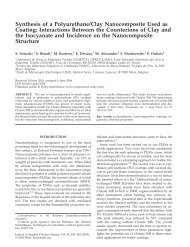
M.-E. Duprez et al. / International Journal of Refrigeration 30 (2007) 873e886875The same two categories may be defined for scrollcompressors.Models [13e16] require the knowledge of pocket volumesand perimeters for every six degrees of rotation, theheight, thickness and pitch of the scrolls that are quitedifficult to obtain. In those models, the whole compressoris divided in several chambers and the compressionprocess is simulated for every gas pockets. It requiresthe evaluation of areas, volumes, pressures, temperaturesand specific volumes for every crank angle. Mass andenergy conservation equations were developed for eachchamber.Model [17] is exclusively thermodynamic and has thesame philosophy as [9e11] used for reciprocating compressors.The refrigerant mass flow rate is affected by a suctiontemperature increase and the compression process is consideredisentropic to the ‘‘adapted’’ pressure and isochoric untilthe discharge pressure.The ARI Standard 540 [18] for positive displacementcompressors recommends the use of third-degree-equationsof 10 coefficients for the calculation of power input, massflow rate of refrigerant, current or compressor efficiency.Those coefficients have no physical meaning so that theextrapolation of the performances outside the operatingrange used for the fitting leads to unrealistic performancesvalues.The purpose of this study is not the development ofa complex model that can relate the performances of thecompressor to its detailed geometry and that could be usedfor technological developments. A simple and thermodynamicallyrealistic model is needed. It should be accurateenough to give mass flow rates and power valuesthat can be used in a global model of a heat pump.Parameters appearing in such a model should be foundin the technical datasheets of the compressors or shouldbe determined in such a way that the calculated massflow rate and electrical power match those given in thesedatasheets.2. Reciprocating compressors2.1. Modelling of reciprocating compressorsThe model developed by Lebrun and coworkers [9e11]has been adapted given the particular requirements mentionedabove.The evolution of the thermodynamic state of the refrigerantthrough the compressor is presented in Fig. 1.The compression process is divided in three steps. Isenthalpic pressure drop in the suction valve (ie1). Isobaric heating up in the suction pipe due to a heattransfer with a fictitious wall at temperature T w(1e2). Isentropic compression (2e3).log pHP = p exLP 0p suc2.1.1. Prediction of the refrigerant mass flow rateThe data are: Evaporation temperature T evap . Condensation temperature T cond . Temperature at the compressor inlet (point i, Fig. 1)T i or superheating DT sup .The parameters of the model are: The suction line diameter d suc . The heat transfer coefficient multiplied by the heattransfer surface during the isobaric heating processin the suction line UA suc . The compressor rotation speed N. The swept volume V s . The ratio between the dead space V d and sweptvolumes 3. The temperature of the fictitious wall T w .Both high and low pressures (HP and LP) can be calculatedfrom the phase change temperatures using Ref. [19](Refprop 7.0 Ò ).LP ¼ p vsat T evap ð1ÞHP ¼ p vsat ðT cond Þð2Þin which p vsat (T) is the saturation vapour pressure law of therefrigerant.Point 0, corresponding to the saturated vapour at lowpressure (Fig. 1), is thus determined.Temperature T i at the inlet of the compressor (point i) iseither directly given or calculated by Eq. (3).T i ¼ T evap þ DT supΔp suc1 2Fig. 1. Diagram (log p, h) of the compression.ð3ÞT i and LP allow the calculation of h i and r i respectively, thespecific enthalpy and density of the refrigerant at the compressorinlet using Ref. [19].The suction pressure p suc (point 1) is given by Eq. (4).p suc ¼ LP Dp suc ð4Þi3iso-sh

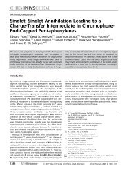
876 M.-E. Duprez et al. / International Journal of Refrigeration 30 (2007) 873e886in which Dp suc is the pressure drop in the suction valve; itcan be deduced from Eq. (5).q m ¼ pd2 suc4pffiffiffiffiffiffiffiffiffiffiffiffiffiffiffiffi2Dp suc r ið5Þpp ex3'3in which: q m is the mass flow rate of refrigerant. d suc is the valve coefficient considered as a pseudodimension.p suc3"2The thermodynamic state of the refrigerant at point 1 isdetermined by Eq. (6) using Ref. [19].h i ðT i ; LPÞ¼h 1 ðT 1 ; p suc Þð6ÞThe temperature at the end of the isobaric heating process(transformation 1e2) T 2 may be deduced from Eq. (7).UA suc DT log suc ¼ q m ðh 2 h 1 Þ ð7Þwith the log-mean difference temperature defined by Eq. (8).DT log suc ¼ ðT w T 1 Þ ðT w T 2 Þð8Þln Tw T1T w T 2In Eqs. (5) and (7), the refrigerant mass flow rate iscalculated by Eq. (9).q m ¼ 1 v 2q vcin which: v 2 is the specific volume of refrigerant at point 2. q vc is the circulated volume flow rate.ð9Þq vc , is determined by Eq. (10).Nq vc ¼ V c ð10Þ60The circulated volume, V c , is the difference betweenvolumes V 2 and V 3 00 defined in the Crank diagram (Fig. 2).V 2 is given by Eq. (11):V 2 ¼ V d þ V s ¼ 3V s þ V sð11ÞThe determination of V 3 00 requires the mass of gas (m 3 00)and the specific volume of refrigerant (v 3 00) at point 3 00(Eq. (12)).V 3 00 ¼ v 3 00m 3 00ð12ÞConsidering the expansion 3 0 3 00 as isentropic, the specificvolume v 3 00 can be calculated knowing the pressurep 3 00 and the specific entropy s 3 00 at point 3 00 .p 3 00 ¼ p sucð13Þs 3 00 ¼ s 3 0ð14Þs 3 0 is calculated knowing the pressure p 3 0 and the specificvolume v 3 0 at point 3 0 .p 3 0 ¼ HPv 3 0 ¼ v 3ð15Þð16ÞIn the same way, considering the compression stepas isentropic, v 3 may be calculated from pressure p 3 andspecific entropy s 3 by:p 3 ¼ HPs 3 ¼ s 2V dm 3 00 in Eq. (12) is calculated by:ð17Þð18Þm 3 00 ¼ V dð19Þv 3 0Assuming that T evap , T cond and T i or DT sup are given, Eqs.(1)e(19) lead to the determination of q m once the parametersof the model are available.The parameters are: The temperature of the fictitious wall T w . The heat transfer coefficient multiplied by the heattransfer surface during the isobaric heating processin the suction line UA suc . The ratio between dead space and swept volumes 3. The diameter of the suction pipe d suc . The rotation speed of the compressor N. The swept volume V s .The last two ones are given by the constructor.The calculation procedure is given in Fig. 3.2.1.2. Prediction of the electrical powerOnce the mass flow rate is calculated, each point in Fig. 1is known.V sV cFig. 2. Crank diagram.V d + V sV

M.-E. Duprez et al. / International Journal of Refrigeration 30 (2007) 873e886877T evapp sucV ds 3'v 3"(11)(1)LPPoint 0 (saturated vapour at LP)(3)p suc initPoint i(4)T 2 inith i(6)T cond Point 2Point 1(2)HPs 2(17), (18)Point 3v 3V s(15), (16)Point 3'm 3' V 2(13), (14)Point 3"T sup ou T i(12)V 3"V cq vcN(10)q m(9)Fig. 3. Mass flow rate calculation.In the previous section, compression (2e3) was supposedto be isentropic. The mechanical power is then written(Eq. (20)).P mecha ¼ q m ðh 3 h 2 Þ ð20ÞThe calculation of the actual electric power consumptionprovided to the compressor requires the knowledge of thefactor (h el h iso-s ), which is the product of the electrical andisentropic efficiencies.This factor allows us to take into account both theelectrical losses and the losses due to the non-isentropiccompression.This term was considered to be a polynomial function ofthe compression ratio (HP/LP) (Eq. (21)).

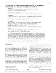
878 M.-E. Duprez et al. / International Journal of Refrigeration 30 (2007) 873e886 6 5 4 HP HP HP HPh el h iso-s ¼ a þb þc þdLP LP LP LP 2 HP HPþ e þ f þ gLP LP 3ð21ÞKnowing the coefficients of the polynomial function it ispossible to calculate the electrical power (Eq. (22)).P elcalc ¼ P mechað22Þh iso-sh elThe prediction of this power consumption requires newparameters (a, b, c, d, e, f, g) but no new operating data:HP and LP were needed for the mass flow rate calculation.2.2. Determination of the parameters2.2.1. Determination of the parameters: massflow rate calculationThe four unknown parameters required for the calculationof the mass flow rate are: T w ,UA suc , 3 and d suc . Theassumption that they are constant for a given compressorand a given refrigerant is made.Their values are found by minimizing the discrepanciesbetween the calculated mass flow rates and the ones providedin the datasheets for given operating conditions (LP,HP, T i , DT sup ).The fictitious wall temperature, T w , has not a significantinfluence on the mass flow rate so its value was set to 50 C.2.2.2. Determination of parameters: electricalpower calculationThe parameters needed for the determination of the electricalpower are the coefficients of the polynomial equationlinking the compression ratio HP/LP to the product of efficiencies(h el h iso-s ). First the isentropic mechanical poweris calculated (Eq. (20)). The ratio P mecha /P electrical is thendeduced from the electrical power provided by the manufacturerin the same operating conditions.This ratio is the product of the electrical and isentropicefficiencies (h el h iso-s ) (Eq. (23)).P mechaP electrical¼ h iso-sh elð23ÞThe evolution of the thermodynamic state of the refrigerantthrough the compressor is presented in Fig. 4.The compression process is divided in three steps. Isobaric heating up in the suction pipe due to a heattransfer with a fictitious wall at temperature T w (1e2). First part of the compression (assumed isentropic,2e3): the gas is compressed until the volume createdby the scrolls matches exhaust volume, V ex . The pressureat point 3 is called ‘‘intermediate pressure, IP’’; itcan be lower or greater than the high pressure. End of the compression at V ex (constant volume) bymass accumulation in the exhaust chamber until thepressure is equal to the exhaust one (3e4).3.1.1. Prediction of the refrigerant mass flow rateThe data are: Evaporation temperature T evap . Condensation temperature T cond . Temperature at the compressor inlet (point 1, Fig. 4)T 1 or superheating DT sup .The parameters of the model are: The temperature of the fictitious wall T w . The heat transfer coefficient multiplied by the heattransfer surface during the isobaric heating processin the suction line UA suc . The swept volume V s . The compressor rotation speed N.Both high and low pressures (HP and LP) can be calculatedfrom the phase change temperatures using Ref. [19].LP ¼ p vsat T evap ð24ÞHP ¼ p vsat ðT cond Þð25Þin which p vsat (T) is the saturation vapour pressure law of therefrigerant.Point 0, corresponding to the saturated vapour at lowpressure (see Fig. 4), is thus determined.A sixth degree polynomial law is used to correlate h el h iso-sto the compression ratio. The values of the parameters aredetermined by an optimization procedure.log pHP = p ex43. Scroll compressors3.1. Modelling of scroll compressorsThe model is an adaptation of the work by Lebrunet al. [17].Iso-VIP3LP = p Iso-ssuc0 1 2hFig. 4. Diagram (log p, h) of the thermodynamic process.

M.-E. Duprez et al. / International Journal of Refrigeration 30 (2007) 873e886879Temperature T 1 at the inlet of the compressor (point 1) iseither directly given or calculated by Eq. (26).Mass flow rate modelT 1 ¼ T evap þ DT supð26ÞPoint 2q mT 1 and LP allow the calculation of h 1 , specific enthalpy ofthe refrigerant at the compressor inlet using Ref. [19].The temperature at the end of the isobaric heating process(transformation 1e2) T 2 may be deduced from Eq. (27).UA suc DT log suc ¼ q m ðh 2 h 1 Þ ð27Þh 2 s 2 v 2 V s V s /V ex p 2 = LP(41)V exs 3h 3 p 3 = IPm sucPoint 4in which q m is the mass flow rate of refrigerant.With the log-mean difference temperature defined byEq. (28).(40)v 3DT log suc ¼ ðT w T 1 Þ ðT w T 2 Þð28Þln Tw T1T w T 2In Eq. (27), the refrigerant mass flow rate is calculated byEq. (29).Point 3T cond(25)HP = p vsat (T cond )s 4IP/LP a bq m ¼ 1 v 2V s Nð29Þin which v 2 is the specific volume of refrigerant at point 2.Assuming T evap , T cond and T 1 or DT sup are given,Eqs. (24)e(29) lead to the determination of q m once theparameters of the model are available.The parameters are: The temperature of the fictitious wall T w . The heat transfer coefficient multiplied by the heattransfer surface during the isobaric heating processin the suction line UA suc . The swept volume V s . The rotation speed of the compressor N.The last two ones are given by the constructor.The calculation procedure is given in Fig. 5.3.1.2. Prediction of the electrical powerThe compression 2e3 is supposed to be isentropic. It occursbetween the low pressure and the intermediate pressurefor which the exhaust volume is obtained. This intermediatepressure, IP, can be either higher or lower than the highpressure.The mechanical work W 23 corresponding to this compressionstep is given by Eq. (30).W 23 ¼ m suc ðu 3 u 2 Þ ð30Þin which:P elcalc(43)(44)pseudo-iso-sFig. 6. Determination of power consumption, diagram. u is the specific internal energy of the gas. m suc is the suctioned mass.T evap(24)T 2 initLPPoint 0 (saturated vapour at LP)Point 2(26)2 V s NPoint 1(29)q mFig. 5. Mass flow rate calculation.T sup or T 1Table 1Characteristics of the studied reciprocating compressorsCompressor Volumic Number Boreflowrate(m 3 h 1 )ofcylinders(mm)Stroke(mm)R1 39.36 4 60 40 5080R2 73.6 4 70 55 9460R3 55.99 4 63.5 50.8 7600R4 70.9 4 68.3 55.6 9150R5 14.9 2 NotavailableNotavailableP (W)(R134a,T cond ¼ 40 C,T evap ¼ 0 C)2162

880 M.-E. Duprez et al. / International Journal of Refrigeration 30 (2007) 873e886Table 2Reciprocating compressors: resultsCompressor Fluid UA suc (W K 1 ) d suc (cm) 3 (%) Discrepancyq m (%)Compressor R1: V s ¼ 452.414 cm 3 , R134a 43.53 2.918 2.50 1.04 3.45N ¼ 1450 t min 1 R404A 48.46 1.772 2.36 0.99 2.37R22 48.91 2.275 4.24 1.02 2.71R12 50 2.457 4.22 1.11 1.66Compressor R2: V s ¼ 845.977 cm 3 , R134a 15.66 2.781 3.41 0.53 1.30N ¼ 1450 t min 1 R404A 19.01 2.043 2.97 0.34 1.16R22 19.77 2.405 4.28 0.50 2.30R12 20.35 2.567 4.18 1.42 0.53Compressor R3: V s ¼ 643.563 cm 3 , R134a 67.93 2.610 4.73 0.80 1.98N ¼ 1450 t min 1 R404A 40.09 2.105 4.59 0.75 1.45R22 5.35 1.962 5.91 0.37 2.24Compressor R4: V s ¼ 814.943 cm 3 , R134a 104.39 3.417 5.11 1.22 1.24N ¼ 1450 t min 1 R404A 95.44 2.678 4.79 1.09 0.86R22 43.97 2.432 5.88 0.39 0.82Compressor R5: V s ¼ 85.64 cm 3 , R134a 13.77 1.221 8.25 1.86 2.79N ¼ 2900 t min 1 R404A 19.38 1.017 6.76 3.06 1.65R407C 22.18 1.132 8.55 1.59 1.23DiscrepancyP (%)The mechanical work during suction, W suc , is given byEq. (31).W suc ¼ V suc LP ð31ÞThe work at the exhaust, W ex , is given by Eq. (32).W ex ¼ V ex HPð32ÞThe total work between points 2 and 4 is obtained by thesummation of the three works (relations (30)e(32)).Volumes V suc and V ex can also be written as Eqs. (33)and (34).V suc ¼ m suc v 2ð33ÞV ex ¼ m suc v 3ð34Þwhich leads to Eq. (35).W ¼ m suc ðu 3 u 2 Þ LPm suc v 2 þ HPm suc v 3 ð35Þgivenu 2 ¼ h 2 LPv 2 ð36Þu 3 ¼ h 3 IPv 3 ð37ÞFig. 7. Compressor R2, R134a q m ¼ f(T evap ).

M.-E. Duprez et al. / International Journal of Refrigeration 30 (2007) 873e886881Fig. 8. Compressor R2, R134a q mcalc /q mconstr ¼ f(T evap ).Eq. (35) becomes Eq. (38).W ¼ m suc ðh 3 h 2 ÞþðHP IPÞm suc v 3 ð38Þwhich leads to the expression of the power (Eq. (39)).P ¼ q m ðh 3 h 2 ÞþðHP IPÞq m v 3 ð39ÞIn Eq. (39) q m is determined by the procedure describedin Section 3.1.1; h 2 is calculated by Ref. [19] knowing thetemperature and pressure conditions at point 2; the highpressure HP is known via relation (24).The specific volume v 3 is calculated by:v 3 ¼ V exm sucð40Þin which: The exhaust volume V ex is determined from the suctionvolume (given by the constructor) and from theratio between this volume and the exhaust volume(V suc /V ex ) which is a parameter of the model. The suctioned mass m suc is calculated by:m suc ¼ V sucð41Þv 2with v 2 calculated by Ref. [19].In Eq. (39), point 3 (h 3 and IP) is known because both thespecific volume v 3 and the specific entropy s 3 are known(Eqs. (40) and (42)).Fig. 9. Compressor R2, R134a P ¼ f(T evap ).

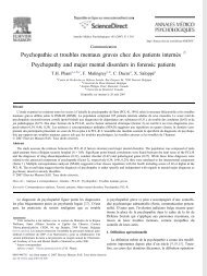
882 M.-E. Duprez et al. / International Journal of Refrigeration 30 (2007) 873e886s 3 ¼ s 2ð42ÞKnowing each term in relation (39), it is possible to calculateP which is the thermodynamic mechanical power (withthe first step considered as isentropic). The calculation ofthe electrical power P elcalc would require the introductionof an isentropic efficiency in the first term of the right-handmember of Eq. (39) as well as an electrical efficiency appliedto each step of the compression. Due to the fact that these twoefficiencies are not applied to the same terms it is not possibleto gather them in one term (h el h iso-s ) as it was the case for reciprocatingcompressors. It appeared that the introduction oftwo new parameters to be dealt with in the optimization procedureled to unrealistic parameter values and to too goodperformances compared to the experimental accuracy ofthe data. As a consequence, given the low influence of thesecond term of the right-hand term of Eq. (39), we only introducedone parameter (applied to the isentropic step) calledthe pseudo-isentropic efficiency and which takes intoaccount both the irreversibilities and the electrical losses.P elcalc ¼ q mðh 3h pseudo-iso-sh 2 ÞþðHP IPÞq m v 3real ð43ÞFor a correct representation of the electrical power, itappeared that this pseudo-isentropic efficiency should beconsidered as a linear function of the ratio IP/LP. v 3real isthe specific volume at the ‘‘real’’ point 3 (non-isentropic).The power calculation procedure is presented in Fig. 6.3.2. Determination of the parameters3.2.1. Determination of the parameters: massflow rate calculationThe two unknown parameters in the mass flow rate predictionare T w and UA suc . The assumption that they are constantfor a given compressor and a given refrigerant is made.Their values are found by minimizing the discrepanciesbetween the calculated mass flow rates and the ones providedin the datasheets for given operating conditions.The fictitious wall temperature, T w , has no significantinfluence on the mass flow rate so that its value was set to50 C.3.2.2. Determination of the parameters:electrical power calculationThe influent parameters in the power prediction arethe ratio between the suction and the exhaust volumes(V suc /V ex ) and the coefficients of the linear law of thepseudo-isentropic efficiency (h pseudo-iso-s ) versus the compressionratio IP/LP.The isentropic efficiency is expressed by Eq. (44).h pseudo-iso-s ¼ a IPLP þ bð44ÞThese three parameters are determined by minimizingthe discrepancies between the calculated electrical powerand the ones provided in the datasheets for given operatingconditions.4. ResultsIn this section, simulation results of mass flow rate andpower for both types of compressors are presented.4.1. Reciprocating compressorsFive reciprocating compressors were studied. Some oftheir characteristics are presented in Table 1 [20e22].Table 2 presents values of the different parameters(UA suc , d suc and 3) and the average discrepancies, respectively,on the mass flow rate and on the electrical powerfor each compressor and each studied fluid.Fig. 10. Compressor R2, R134a P calc /P constr ¼ f(T evap ).

M.-E. Duprez et al. / International Journal of Refrigeration 30 (2007) 873e886883Table 3Characteristics of the studied scroll compressorsCompressorVolumic flowrate (m 3 h 1 )S1 25 3770S2 36 5420S3 8.6 1340S4 35.56 5500S5 43.5 6866P (W) (R134a,T cond ¼ 40 C, T evap ¼ 0 C)The model is very good at predicting mass flow rate andpower consumption of reciprocating compressors: averagediscrepancies are lower than 3%. In most cases, the pointsfor which the discrepancy is higher than 5% correspond toevaporation temperatures lower than 20 C and/or condensationtemperature higher than 60 C. In residential heatpumps, those ranges of temperatures are rare.Figs. 7 and 8 present, respectively, the evolution of themass flow rate (calculated and given by the manufacturer)and the related discrepancy as a function of the evaporationtemperature for different condensation temperatures (30, 40and 50 C).For evaporation temperatures higher than 20 C thediscrepancy on the mass flow rate is lower than 1%.Figs. 9 and 10 present, respectively, the evolution of theelectrical power (calculated and given by the manufacturer)and the related discrepancy as a function of the evaporationtemperature for different condensation temperatures (30, 40and 50 C).For evaporation temperatures higher than 20 C thediscrepancy on the mass flow rate is lower than 2.5%.4.2. Scroll compressorsFive reciprocating compressors were studied. Some oftheir characteristics are presented in Table 3 [20e22].Table 4 presents the values of the different parameters(UA suc , V suc /V ex , a and b) and the average discrepancies,respectively, on the mass flow rates and on the electricalpowers for each compressor and each fluid.The model is very good at predicting mass flow rate andpower of scroll compressors. The mean discrepancies arelower than 3.5%. In most cases, points for which discrepancyis higher than 5% correspond to evaporation temperatureslower than 20 C and/or condensation temperaturehigher than 60 C. In the residential heat pumps, thoseranges of temperatures are rare.Figs. 11 and 12 present, respectively, the evolution ofmass flow rate and the discrepancy on this mass flow rateas a function of the evaporation temperature for differentcondensation temperatures.The discrepancy on the mass flow rate is generally lowerthan 5%. It can reach nearly 10% for high condensation temperatures(55 and 60 C).Figs. 13 and 14 present, respectively, the evolution ofpower and the discrepancy on this power as a function ofthe evaporation temperature for different condensationtemperatures.Table 4Scroll compressors: resultsCompressor Fluid UA suc(W K 1 )V suc /V ex(e)a (e) b (e) Discrepancyq m (%)Compressor S1: V s ¼ 143.678 cm 3 , R134a 19.01 2.379 0.777 2.585 1.70 1.12N ¼ 2900 t min 1 R404A 48.36 2.165 0.010 0.682 1.57 0.19R407C 42.06 2.219 0.312 1.463 2.31 0.46R22 60.33 2.187 0.671 2.329 2.21 0.59Compressor S2: V s ¼ 206.897 cm 3 , R134a 26.99 2.378 0.772 2.570 1.74 1.12N ¼ 2900 t min 1 R404A 69.59 2.166 0.003 0.698 1.59 0.16R407C 59.49 2.220 0.316 1.473 2.31 0.46R22 87.09 2.189 0.677 2.345 2.18 0.59Compressor S3: V s ¼ 47.778 cm 3 , R134a 5.39 2.302 0.473 1.766 1.47 0.85N ¼ 3000 t min 1 R404A 18.97 2.089 0.320 1.361 2.95 1.02R22 22.67 2.128 0.642 2.142 3.15 2.26R407C 17.44 2.156 1.152 3.302 1.97 1.21Compressor S4: V s ¼ 197.556 cm 3 , R134a 107.02 2.637 0.134 1.022 2.32 0.53N ¼ 3000 t min 1 R404A 44.93 2.667 0.113 0.954 2.95 1.49R22 131.05 2.937 0.215 1.422 2.78 1.24R407C 146.36 2.799 0.194 1.273 2.95 1.08Compressor S5: V s ¼ 24.99 cm 3 , R134a 34.64 2.466 0.826 2.752 2.02 0.66N ¼ 2900 t min 1 R22 62.43 2.293 0.579 2.148 1.84 0.58R407C 99.14 2.239 0.465 1.787 2.23 0.55DiscrepancyP (%)

884 M.-E. Duprez et al. / International Journal of Refrigeration 30 (2007) 873e886Fig. 11. Compressor S3, R404A q m ¼ f(T evap ).The discrepancy on the power is also generally lowerthan 5%. It can be higher than 5% for low condensation temperatures(10 and 15 C).5. ConclusionIn this paper, simple and thermodynamically realisticmodels of the two types of compressors found in the residentialheat pumps (reciprocating and scroll compressors) havebeen presented. Those models calculate the mass flow rate ofrefrigerant and the power consumption from the knowledgeof operating conditions (phase change temperatures andrefrigerant temperature at the inlet of the compressor orsuperheating) and different parameters.Parameters appearing in the models are found in the technicaldatasheets of the compressors or they are fitted in sucha way that the calculated mass flow rate and electrical powermatch those given in these datasheets.The reciprocating compressor model requires the knowledgeof six parameters. Two of them are given in the datasheets:the swept volume (V s ) and the compressor rotationspeed (N). The last four are: the temperature of the fictitiouswall (T w ) which is actually set to a constant value (50 C),the global heat transfer coefficient at suction (UA suc ), thediameter of the suction pipe (d suc ) and the ratio betweenthe dead space and the swept volume (3). Those three parametershave to be fitted in order that the calculated mass flowrates match the ones given in the datasheets. The determinationof the powers requires the knowledge of the seven coefficientsof the polynomial law relating the product of theelectrical and isentropic efficiencies to the compressionratio.This model has been tested on five compressors. Themean discrepancies values on the determination of,respectively, mass flow rate and power consumption are1.15 and 2.04% (R134a), 1.38 and 1.43% (R404A),Fig. 12. Compressor S3, R404A q mcalc /q mconstr ¼ f(T evap ).

M.-E. Duprez et al. / International Journal of Refrigeration 30 (2007) 873e886885Fig. 13. Compressor S3, R404A P ¼ f(T evap ).0.51 and 1.86% (R22), 1.27 and 1.09% (R12), 1.59 and1.23% (R407C).The scroll compressor model requires the knowledge ofseven parameters. Two of them are given in the datasheets:the swept volume (V s ) and the compressor rotation speed(N). The last five are: the temperature of the fictitious wall(T w ) which is actually set to a constant value (50 C), theglobal heat transfer coefficient at suction (UA suc ), the ratiobetween the swept volume and the exhaust volume (V suc /V ex ) and the two parameters a and b of the linear law ofthe pseudo-isentropic efficiency. Those four parametershave to be fitted in order that the calculated mass flow rateand power matches those given in the datasheets. UA suc isfitted using the mass flow rate data while the three otherparameters (V suc /V ex , a, and b) are fitted using powerconsumption data.This model has been tested on five compressors. Themean discrepancy values on mass flow rate and power are1.89 and 0.76% (R134a), 2.76 and 1.12% (R404A), 2.39and 0.91% (R407C), 2.59 and 1.31% (R22).Although, it was not hinted in this paper those models failat predicting correct outlet temperatures (up to 50 C differencedepending on the compressor and fluid, usually the differenceis around 20e25 C). So the same philosophy at theoutlet than at the inlet (taking into account a heat transferwith the fictitious wall) should be applied. The determinationof the global heat transfer coefficient at the exhaust (UA ex )requires values of exhaust temperature or values of heatflow rate at the condenser. As temperature T w has a significantinfluence on the outlet temperature of the compressor, itseems interesting to make it vary with the phase changetemperatures and power consumption of the compressor.Fig. 14. Compressor S3, R404A P calc /P constr ¼ f(T evap ).

886 M.-E. Duprez et al. / International Journal of Refrigeration 30 (2007) 873e886It is also possible to determine one set of parameters forall the refrigerants and for a given compressor.It must also be noticed that the isentropic and electricalefficiencies that are used for the determination of the powerhave no real physical sense (the use of parameters with physicalsense leads to an over-parameterised model). This lackof physical sense can explain the higher discrepancies athigh temperatures.References[1] H. Rivoalen, Heat Pump Market Overview in Europe, HandsonExperience with Heat Pumps in Buildings, Workshop ReportHPC-WR-23, Arnhem, The Netherlands, October 2001.[2] C.D. Pérez-Segarra, J. Rigola, A. Oliva, Modelling andnumerical simulation of the thermal and fluid dynamic behaviourof hermetic reciprocating compressors. Part 1: theoreticalbasis, HVAC & R Research 9 (2) (2003) 215e235.[3] J. Rigola, C.D. Pérez-Segarra, A. Oliva, Modelling andnumerical simulation of the thermal and fluid dynamic behaviourof hermetic reciprocating compressors. Part 2: experimentalinvestigation, HVAC & R Research 9 (2) (2003)237e249.[4] J. Rigola, C.D. Pérez-Segarra, A. Oliva, Parametric studies onhermetic reciprocating compressors, International Journal ofRefrigeration 28 (2005) 253e266.[5] J. Rigola, C.D. Pérez-Segarra, A. Oliva, J.M. Serra, M.Escribà, J. Pons, Advanced numerical simulation model ofhermetic reciprocating compressors, Parametric study anddetailed experimental validation, in: Proceedings of the 15thInternational Compressor Engineering Conference at PurdueUniversity, USA, 2000, pp. 23e30.[6] J.M. Corberan, J. Gonzalvez, J. Urchueguía, A. Calas, Modellingof refrigeration compressors, in: Proceedings of the 15thInternational Compressor Engineering Conference at PurdueUniversity, USA, 2000, pp. 571e578.[7] M.L. Todescat, F. Fagotti, Thermal energy analysis inreciprocating hermetic compressors, in: Proceedings of theInternational Compressor Engineering Conference at PurdueUniversity, USA, 1992, pp. 1419e1428.[8] P. Popovic, H.N. Shapiro, A semi-empirical method for modellinga reciprocating compressor in refrigeration systems,ASHRAE Transactions 101 (1995) 367e382.[9] E. Winandy, O.C. Saavedra, J. Lebrun, Simplified modellingof a open-type reciprocating compressor, International Journalof Thermal Science 41 (2002) 183e192.[10] M. Grodent, J. Lebrun, E. Winandy, Simplified modelling ofan open-type reciprocating compressor using refrigerantsR22 et R410A. 2nd part: model, in: Proceedings of the 20thInternational Congress of Refrigeration, Sidney, vol. 3, 1999(paper 800).[11] C. Hannay, J. Lebrun, D. Negoiu, E. Winandy, Simplifiedmodelling of an open-type reciprocating compressor usingrefrigerants R22 et R410A. 1st part: experimental analysis,in: Proceedings of the 20th International Congress of Refrigeration,Sidney, vol. 3, 1999 (paper 657).[12] D.I. Jähnig, D.T. Reindl, S.A. Klein, A semi-empiricalmethod for representing domestic refrigerator/freezer compressorcalorimeter test data, ASHRAE Transactions 106(2000) 122e130.[13] J.-L. Caillat, S. Ni, M. Daniels, A computer model for scrollcompressors, in: Proceedings of the International CompressorEngineering Conference at Purdue University, USA, 1988,pp. 47e55.[14] Y. Chen, N.P. Halm, E.A. Groll, J.E. Braun, Mathematicalmodelling of scroll compressors. Part I: compression processmodelling, International Journal of Refrigeration 25 (2002)731e750.[15] Y. Chen, N.P. Halm, E.A. Groll, J.E. Braun, Mathematicalmodelling of scroll compressors. Part II: overall scroll compressormodelling, International Journal of Refrigeration 25(2002) 751e764.[16] C. Shein, R. Radermacher, Scroll compressor simulationmodel, Journal of Engineering for Gas Turbines and Power123 (2001) 217e225.[17] E. Winandy, O.C. Saavedra, J. Lebrun, Experimental analysisand simplified modelling of a hermetic scroll refrigerationcompressor, Applied Thermal Engineering 22 (2002)107e120.[18] Performance Rating of Positive Displacement RefrigerantCompressors and Compressor Units, ARI Standard 504,Air-Conditioning and Refrigeration Institute, Arlington,2004.[19] REFPROP, NIST Standard Reference Database 23, Version 7.0.[20] Bitzer e Software, .[21] Copeland Selection Software Select, .[22] Products datasheets, .