Solutions to Tutorial Sheet 1: Mainly revision 1. Given the expansion ...

Solutions to Tutorial Sheet 1: Mainly revision1. Given the expansion of an arbitrary wavefunction or state vector as a linear superpositionof eigenstates of the operator ÂΨ(r, t) = ∑ ic i (t)u i (r) or |Ψ, t〉 = ∑ ic i (t) |u i 〉use the orthonormality properties of the eigenstates to prove that∫c i (t) = u ∗ i (r)Ψ(r, t) d 3 r or c i (t) = 〈u i |Ψ, t〉Work through the proof in both wavefunction and Dirac notations.Firstly in wavefunction notation the expansion is:Ψ(r, t) = ∑ ic i (t)u i (r)Multiply both sides by u ∗ j(r) and integrate over all space:∫u ∗ j(r)Ψ(r, t) d 3 r = ∑ i∫c i (t)u ∗ j(r) u i (r) d 3 r = ∑ ic i (t) δ ji = c j (t)where we have used the orthonormality property of the eigenfunctions:∫u ∗ j(r)u i (r) d 3 r = δ jiand the so-called sifting property of the Kronecker delta:∑c i (t) δ ji = c j (t)iRelabelling the free index j → i gives the desired result:∫c i (t) = u ∗ i (r)Ψ(r, t) d 3 rIn Dirac notation we start from the expansion:|Ψ, t〉 = ∑ ic i (t) |u i 〉and take the scalar product of both sides with the bra vector 〈u j | to give〈u j |Ψ, t〉 = ∑ ic i (t) 〈u j |u i 〉 = ∑ ic i (t) δ ji = c j (t)using the orthonormality property 〈u j |u i 〉 = δ ji as before.1

The state |Ψ, t〉 is said to be normalised if 〈Ψ, t|Ψ, t〉 = 1. Show that this implies that∑|c i (t)| 2 = 1iHint: use the expansion |Ψ, t〉 = ∑ ic i (t)|u i 〉 and the corresponding conjugate expansion〈Ψ, t| = ∑ jc ∗ j(t)〈u j |.Substituting for 〈Ψ, t| and |Ψ, t〉 in 〈Ψ, t|Ψ, t〉 we find〈Ψ, t|Ψ, t〉 = ∑ ∑c ∗ j(t)c i (t)〈u j |u i 〉 = ∑ ∑c ∗ j(t)c i (t)δ ji = ∑j ij ii|c i (t)| 2where we have used the orthonormality of the eigenbasis 〈u j |u i 〉 = δ ji and the siftingproperty of the Kronecker delta. Thus we have the result quoted in Lecture 1:∑|c i (t)| 2 = 1iIf the expectation value 〈Â〉 t = 〈Ψ, t|Â|Ψ, t〉, show by making use of the same expansionsthat〈Â〉 t = ∑ |〈u i |Ψ, t〉| 2 A iiand give the physical interpretation of this result.The suggested expansion of the state vector is, in Dirac notation,|Ψ, t〉 = ∑ ic i (t)|u i 〉 where c i (t) = 〈u i |Ψ, t〉and, correspondingly,〈Ψ, t| = ∑ jc ∗ j(t)〈u j |Substituting for |Ψ, t〉 and 〈Ψ, t| in the expression for the expectation value gives〈Â〉 t = ∑ j∑ic ∗ j(t)c i (t)〈u j |Â|u i〉 = ∑ jwhere we have used the eigenvalue equation for Â:Â|u i 〉 = A i |u i 〉∑ic ∗ j(t)c i (t)A i 〈u j |u i 〉We again use the orthonormality of the eigenbasis 〈u j |u i 〉 = δ ji to write〈Â〉 t = ∑ j∑ic ∗ j(t)c i (t)A i δ ji = ∑ i|c i (t)| 2 A i = ∑ i|〈u i |Ψ, t〉| 2 A iwhich is the desired result. As discussed in lectures, the interpretation is that |c i (t)| 2is the probability of getting the result A i in a measurement of the observable A, andthe mean value of a set of repeated measurements of A is just a sum over the possiblevalues weighted by the probabilities of obtaining them.2

2. The observables A and B are represented by operators  and ˆB with eigenvalues {A i },{B i } and eigenstates {|u i 〉}, {|v i 〉} respectively, such that|v 1 〉 = { √ 3 |u 1 〉 + |u 2 〉}/2|v 2 〉 = {|u 1 〉 − √ 3 |u 2 〉}/2|v n 〉 = |u n 〉, n ≥ 3.Show that if {|u i 〉} is an orthonormal basis then so is {|v i 〉}.This problem is designed to test your understanding of measurement and wavefunctioncollapse.Orthonormality of the two bases means that〈u i |u j 〉 = δ ij and 〈v i |v j 〉 = δ ijGiven the expressions for |v 1 〉 and |v 2 〉 in terms of |u 1 〉 and |u 2 〉 we see that〈v 1 |v 1 〉 = 1 (√3〈u1 | + 〈u 2 | ) ( √3|u1 〉 + |u 2 〉 )4= 1 (3〈u1 |u 1 〉 + √ 3〈u 1 |u 2 〉 + √ 3〈u 2 |u i 〉 + 〈u 2 |u 2 〉 ) = 1 (3 + 0 + 0 + 1) = 144as it should. Similarly,〈v 1 |v 2 〉 = 1 (√3〈u1 | + 〈u 2 | ) ( |u 1 〉 − √ 3|u 2 〉 )4= 1 (√3〈u1 |u 1 〉 − 3〈u 1 |u 2 〉 + 〈u 2 |u i 〉 − √ 3〈u 2 |u 2 〉 ) = 1 (√ √ )3 − 0 + 0 − 3 = 044By the same methods you can show that 〈v 2 |v 2 〉 = 1 and 〈v 2 |v 1 〉 = 0 so that the relationsbetween |v 1 〉, |v 2 〉 and |u 1 〉, |u 2 〉 are consistent with both bases being orthonormal(for n ≥ 3 it is trivial).A certain system is subjected to three successive measurements:(1) a measurement of A followed by(2) a measurement of B followed by(3) another measurement of AShow that if measurement (1) yields any of the values A 3 , A 4 , . . . then (3) gives thesame result but that if (1) yields the value A 1 there is a probability of 5 that (3) will8yield A 1 and a probability of 3 that it will yield A 8 2. What may be said about thecompatibility of A and B ?If measurement (1) yields any of the eigenvalues A 3 , A 4 , . . . then the state of the systemimmediately afterwards is the corresponding eigenstate |u 3 〉, |u 4 〉, . . . of the operator Â.But |u 3 〉 = |v 3 〉 etc. and so measurement (2) is made with the system in an eigenstateof ˆB, guaranteeing the outcome of (2) and leaving the state of the system unchanged,since for n ≥ 3, |u n 〉 = |v n 〉. Thus measurement (3) is certain to yield the same resultas (1).3

If measurement (1) yields the result A 1 , however, the system is forced into the state|u 1 〉 so that measurement (2), of the observable B, is made with the system in the state|u 1 〉. Inverting the given equations shows that|u 1 〉 = { √3|v1 〉 + |v 2 〉 } /2|u 2 〉 = { |v 1 〉 − √ 3|v 2 〉 } /2The first of these is just the expansion of |u 1 〉 in the eigenbasis of ˆB and the coefficientsare the probability amplitudes from which we can compute the probabilities of gettingthe various possible values of B:prob of B 1 =√ 32= 3 ∣ 2 ∣ 4prob of B 2 =12∣ ∣ = 1 2 4Suppose that we get the result B 1 . The wavefunction has collapsed onto the correspondingeigenstate of ˆB, that is |v 1 〉. But we know that|v 1 〉 = { √ 3 |u 1 〉 + |u 2 〉}/2which is the expansion of |v 1 〉 in the eigenbasis of Â, enabling us to compute theprobabilities of getting the various possible values of A:prob of A 1 =√ 32= 3 ∣ 2 ∣ 4prob of A 2 =12∣ ∣ = 1 2 4On the other hand, if we get the result B 2 from measurement (2), the system is left inthe state |v 2 〉 and|v 2 〉 = {|u 1 〉 − √ 3 |u 2 〉}/2so that in this case when we make measurement (3)prob of A 1 =prob of A 2 =12∣ ∣ = 1 2 4√ 32= 3 ∣ 2 ∣ 4Thus the probability of getting the result A 1 in measurement (3), irrespective of theoutcome of measurement (2), is given by(prob that (2) gives B 1 ) × (prob that (3) gives A 1 given outcome B 1 in (2))+(prob that (2) gives B 2 ) × (prob that (3) gives A 1 given outcome B 2 in (2))= 3 4 × 3 4 + 1 4 × 1 4 = 5 84

Since (3) can only give A 1 or A 2 , the probability of getting A 2 is 3/8.We can represent the situation by a probability tree:Measurement (1):Measurement (2):Measurement (3):A 13/4 1/4B 1 B 23/4 1/4 1/43/4A 1 A 2 A 1A 2Â and ˆB are not compatable operators, even though many of their eigenstates are thesame.3. The normalised energy eigenfunction of the ground state of the hydrogen atom (Z = 1)isu 100 (r) = R 10 (r)Y 00 (θ, φ) = C exp(−r/a 0 )where a 0 is the Bohr radius and C is a normalisation constant. For this state(a) Calculate the normalisation constant, C, by noting the useful integral∫ ∞exp(−br) r n dr = n!/b n+1 , n > −10Alternatively, you can use the computer algebra program Maple if you know howto!The normalisation condition is as usual∫u ∗ 100(r)u 100 (r) d 3 r = 1which in spherical polar coordinates gives∫ 2πφ=0∫ πθ=0∫ ∞r=0|C| 2 exp(−2r/a 0 )r 2 sin θdrdθdφ = 1The φ integration gives 2π, whilst the θ integration gives 2 so that∫ ∞4π|C| 2 exp(−2r/a 0 )r 2 dr = 1We use the given integration formula and we find that∫0exp(−2r/a 0 )r 2 dr = 2!( ) a0 3a 3=02 4Making the usual convention that the normalisation constant C is real and positivegivesC = √1πa 3 0; u 100 (r) = (πa 3 0) −1/2 exp(−r/a 0 )Maple can be used to evaluate the required integral (and related integrals which occurin the subsequent parts of the question).5

assume(a>0);> int(exp(-2*r/a)*r*r,r=0..infinity);(b) Determine the radial distribution function, D 10 (r) ≡ r 2 |R 10 (r)| 2 , and sketch itsbehaviour; determine the most probable value of the radial coordinate, r, and theprobability that the electron is within a sphere of radius a 0 ; recall that Y 00 (θ, φ) =1/ √ 4π; again, you can use Maple to help you if you know how;Recall thatso thatu nlm (r) = R nl (r) Y lm (θ, φ)u 100 (r) = R 10 (r) Y 00 (θ, φ) = 1 √4πR 10 (r)Using the result for u 100 (r) from the previous part of the question,D 10 (r) ≡ r 2 |R 10 (r)| 2 = 4r2a 3 0exp(−2r/a 0 )To plot the radial distribution using Maple, use the following Maple command:> plot(4*r*r*exp(-2*r),r=0..3);This will produce a graph with a 0 scaled to 1.D 10 (r) dr is the probability of finding the electron between r and r + dr, so that themost probable value of r corresponds to the maximum of the distribution, which maybe found by differentiation with respect to r;dD 10dr= 8r exp(−2r/aa 3 0 ) − 8r20a 4 0exp(−2r/a 0 ) = 8r (aa 4 0 − r) exp(−2r/a 0 )0Thus the derivative vanishes at the origin and at r = a 0 , the latter corresponding tothe maximum of D 10 .The following piece of Maple finds the points at which the derivative vanishes:> assume(a>0);> d:=4*r*r*exp(-2*r/a)/a**3;> dprime:=diff(d,r);> solve({dprime=0},{r});The probability that the electron is within a sphere of radius a 0 is given by integratingthe radial probability distribution from r = 0 to r = a 0 :∫ a00D 10 (r) dr = 4 a 3 0∫ a00r 2 exp(−2r/a 0 ) drUnfortunately, the given integral doesn’t help because here the upper limit is a 0 andnot ∞. However, integrating by parts or using Maple yields the resultThe Maple isprobability = 1 − 5e −2 = 0.326

d:=4*r*r*exp(-2*r/a)/a**3;> prob:=int(d,r=0..a);> evalf(prob);(c) Calculate the expectation value of r;∫〈r〉 =Using the given integral, or Maple,u ∗ 100(r)r u 100 (r) d 3 r = 4π ∫ ∞r 3 exp(−2r/aπa 3 0 ) dr0 0〈r〉 = 4 a 3 03!( ) a0 43 =2 2 a 0So, the mean value of r is 50% larger than the most probable value. This is due to thelong “tail” of the wavefunction.(d) Calculate the expectation value of the potential energy, V (r);〈V (r)〉 = − e24πɛ 0∫= − e24πɛ 04π 1= − e24πɛ 04a 3 0= − e24πɛ 0 a 0u ∗ 100(r) 1 r u 100(r) d 3 rπa 3 0( a02∫ ∞0r exp(−2r/a 0 ) dr) 2from the given integral(e) Calculate the uncertainty, ∆r, in r.The uncertainty is defined by∆r ≡√〈r 2 〉 − 〈r〉 2so we need to compute 〈r 2 〉:〈r 2 〉 =∫= 4π 1= 4 a 3 0= 3a 2 0u ∗ 100(r) r 2 u 100 (r) d 3 r∫ ∞πa 3 0 0( ) a0 54!2r 4 exp(−2r/a 0 ) drThus∆r =√3a 2 0 − (1.5a 0 ) 2 =√32 ≈ 0.87a 07

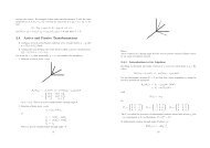
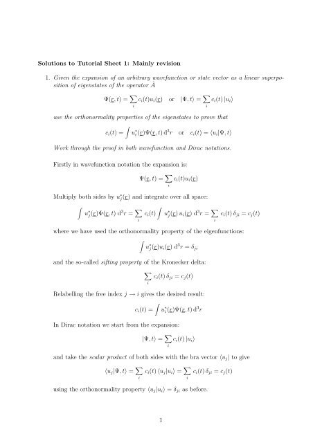
4. At t = 0, a particle has a wavefunction ψ(x, y, z) = A z exp[−b(x 2 + y 2 + z 2 )], whereA and b are constants.(a) Show that this wavefunction is an eigenfunction of ˆL 2 and of ˆL z and find the correspondingeigenvalues. Hint: express ψ in spherical polars and use the sphericalpolar expressions for ˆL 2 and ˆL z .ˆL 2 = −¯h 2 [ 1sin θˆL z = −i¯h ∂∂φ(∂sin θ ∂ )+ 1∂θ ∂θ sin 2 θFirst note that x 2 + y 2 + z 2 = r 2 and z = r cos θ, so thatu(r, θ, φ) = Ar cos θ exp(−br 2 )∂ 2 ]∂φ 2In spherical polars,ˆL 2 = −¯h 2 [ 1sin θ(∂sin θ ∂ )+ 1∂θ ∂θ sin 2 θ∂ 2 ]∂φ 2Since u is actually independent of φ, we can ignore the second term when we apply ˆL 2to the wavefunction u and note that1 ∂(sin θ ∂ )sin θ ∂θ ∂θ cos θ = 1 ∂ (− sin 2 θ ) = −2 cos θsin θ ∂θThusˆL 2 u(r, θ, φ) = 2¯h 2 Ar cos θ exp(−br 2 ) = 2¯h 2 u(r, θ, φ)so that u(r, θ, φ) is an eigenfunction of ˆL 2 with eigenvalue 2¯h 2 . Writing 2¯h 2 = l(l+1)¯h 2 ,we see that the orbital angular momentum quantum number l = 1.We have already noted that u(r, θ, φ) is independent of φ which tells us immediatelythat it is an eigenfunction of ˆL z belonging to eigenvalue m = 0. Explicitly, we notethat in spherical polar coordinates,ˆL z = −i¯h ∂∂φso that ˆL z u(r, θ, φ) = 0. A short cut to the answer is to note that u(r, θ, φ) ∝ Y 10 (θ, φ)and hence l = 1 and m = 0.(b) Sketch the wavefunction, e.g. with a contour plot in the x=0 plane.The function is zero at the origin. It has positive and negative lobes pointing aongthe z-axis, decaying away to zero far from the origin. In fact, it looks a bit like ahydrogenic p-orbital (l = 1), though it isn’t quite the same.8

zPositive lobe+Zero for z=0yNegative lobe_(c) Can you identify the Hamiltonian for which this is an energy eigenstate ?The given function is an eigenfunction of the 3-dimensional isotropic simple harmonicoscillator with b related to the mass m and angular frequency ω through b = mω/2¯h.It is the state with n x = n y = 0 and n z = 1.note: the 2007 version asked you to identify a physical system - this is rather challenging,an “atom trap” can capture single particles, which won a 1997 Nobel Prize forChu, Cohen-Tannoudji and Phillips, and another in 2001 for Wieman, Ketterle andCornell who trapped millons of Rubidium atoms in the same quantum state, forminga Bose Condensate. Optical tweezers are a method by which a particle can be trappedin a laser cavity. If you don’t know about this stuff, look it up.More esoterically (see 2007 exam), a neutrino trapped in the gravitational field of aconstant density planet is a possibility!9