Chapter 10 Design Optimization A Prototype Problem (I)
Chapter 10 Design Optimization A Prototype Problem (I)
Chapter 10 Design Optimization A Prototype Problem (I)

Create successful ePaper yourself
Turn your PDF publications into a flip-book with our unique Google optimized e-Paper software.
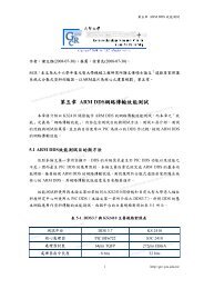
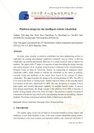
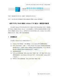
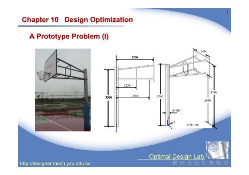
<strong>Chapter</strong> <strong>10</strong> <strong>Design</strong> <strong>Optimization</strong>1A <strong>Prototype</strong> <strong>Problem</strong> (I)2250<strong>10</strong>00125035002000370037502950D=200yxzunit: mm
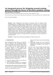
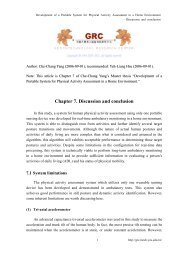
A <strong>Prototype</strong> <strong>Problem</strong> (II)2 FEM analysis4L33L22L13L<strong>10</strong>L7L4L15 816L24L14 L2012L11L12715L19 L2311L17L25L18L9614L8<strong>10</strong>L21 L22L16 L5 13L659MXMNMXL1Y1 XZF=3200NYMN XZδ max =48.55mmYXZσ max =306.78MPa
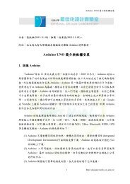
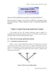
A <strong>Prototype</strong> <strong>Problem</strong> (III)3 Adding two reinforced beams:abab
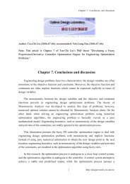
A <strong>Prototype</strong> <strong>Problem</strong> (IV)4 <strong>Design</strong> requirements• To minimize the maximum deflection of the structure.• The maximum stress should be lower than the allowable stress.• The length of the complimentary beam should be less than 1.0m.min. δ max (a, b)s.t.σ max ( a,b)≤Sya 2 + b2 =L Objective function and constraints <strong>Design</strong> variables and design parameters Inequality constraint and equality constraint
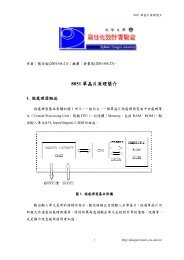
Solving the <strong>Prototype</strong> <strong>Problem</strong> (II)6 1.41% error with FEA Sensitivity analysis: 1%perturbation of designvariable a causes only0.02% variation in δ max . It is a “robust design”.a=0.47
Interpreting the <strong>Optimization</strong> Result (I)7 Feasible domain Interior optimum Inactive constraint
Interpreting the <strong>Optimization</strong> Result (II)8 Boundary optimum Active constraint
<strong>Design</strong> <strong>Optimization</strong><strong>10</strong> In mechanical design process, a designer often faces all kinds of designdecisions to improve performance of the product or to meet certain designrequirements. A designer generates a design prototype, evaluate the design prototype, thenmodify the design prototype according to his/her evaluation. Very often, this is done in a “trial-and-error” manner. The process is inefficient,and the result is often a “satisfactory design”, instead of an “optimal design”. In the design optimization process, A design problem is expressed in amathematical optimization model. The model is then solved by a computerizednumerical optimization algorithm to get the optimal design. <strong>Design</strong> optimization is a structured way of thinking to help designerssystematically construct the design problem, and search, select the best design.
To “select” the “best” “possible” design11 Select: A designer has the flexibility to select the values of the design variableswhich will affect the performance of the design. Best: A designer has to construct a performance index or objective functionaccording to the design requirements to define what is the best design. Possible: The best design is often not possible. A designer has to search for thebest design under the constraints such as material, space, time, cost, etc. <strong>Design</strong> optimization can also be a qualitative decision process. Here we assumethat the design variables, objective function, and constraints can all beexpressed quantitatively. General procedure for quantitative design optimization: To establish theoptimization model To solve the optimization model To interpret theoptimization results
(1) What are the <strong>Design</strong> Variables?12lrF Radius r and length l are design variables. If the designer can freely choose the material, the material properties E and Ware design variables too. E and W cannot be any arbitrary value, they are discrete design variables. Discrete variables, including integer variables and binary variables, are morecommon than continuous variables in engineering design optimizationproblems.
(2) What are the <strong>Design</strong> Parameters?13lrF If the material is given, the material properties E and W becomes design parameters. <strong>Design</strong> parameters are often given by design specifications and cannot cbe changedby the designer, for example, the load F. <strong>Design</strong> parameters may change underdifferent design specifications. Here we use capital letters for design parameters, small letters for design variables. Quantities that will never change, such as circumferential ratio or speed of light,are call constants.
(3) Choose One <strong>Design</strong> Requirement as the Objective Function14lr List the design requirements: light weight, low stress, high rigidity. There are often “trade-off” between different design requirements. We can combineseveral design requirements to form a multi-objective optimization problem. The designer can choose one design requirement as the objective function and use theother design requirements as constraints.F
(4) Construct the Mathematical Optimal <strong>Design</strong> Model15min.s.t σmaxδweightr,l ( )( r,l) ≤ Smax( r,l) ≤ D (1)lrmin.s.t.Wπr2 lFlr ≤ Si3Fl≤ D3Ei4πri =4l ≥ LT( , l,i) ∈℘ (7)F Wπ is the scaling factor i is an intermediate variable Inequality constraint, equalityconstraint, and set constraint Positive finite domain:r ℘≡ { x 0 < x < ∞,i 1,......, n} (6)i i=
Standard Form of the Mathematical Optimal <strong>Design</strong> Model16min.Wπr2 lmin.f= Wπr2ls.t.Flr ≤ Si3Fl≤ D3Ei4πri =4l ≥ LT( r,l,i) ∈℘ (7)min.s.t.f ( x)g(x)≤ 0h ( x)=0nx ∈℘⊂ R(8)Flrs.t. g1 = − S ≤ 0i3Flg2= − D ≤ 03Eihπr= i −441=g3 = L − l ≤ 00T3( r,l,i) ∈℘⊂ R (9)
Example 1. Optimal <strong>Design</strong> Model for a Vehicular Jack(I)17min. V =8LBHs.t. H ≤ H maxFor minimum volumeAssembly considerationWFmax≤P crPrevent from bucklingA= CπEIP cr2LEuler equationθI =BH123Moment of inertia4Fθ ≥ WmaxsinminmaxMax. weight the jack can lift2Lsinθ≤ Kmin1To be put under the car2Lsinθ≥ Kmax2Max. height the jack can lift
Example 1. Optimal <strong>Design</strong> Model for a Vehicular Jack(II)18min. v = 8lbhs.t.g1= h − Hmax≤0Wgh2= fmax− Pcr≤CπEil021= Pcr− =20Aθhbh1232= i − =0g3 = 4 fmaxsinθmin−Wmax= 0g4= 2lsinθmin− K1≤0g5 = −2lsinθmax+ K2≤ 0(<strong>10</strong>)
A Double Spring Example (I)19 The spring will balance at the position where thesystem has the lowest potential energy.PE=+1212KK21 Analytical Method:12⎡⎢⎣∂PE∂x1⎡⎢⎣=x21x0++( L − x )12( L + x ) − L ⎤ − P x − P x (11)2∂PE∂x2=220 Numerical algorithms are all iterative numericalmethods.2− L ⎤1⎥⎦22⎥⎦21122L1= <strong>10</strong>cmL 2 = <strong>10</strong>cmAK 1 = 8N/cmP 2 = 5NP 1 = 5NK2= 1N/cm1
Structure of an <strong>Optimization</strong> Algorithm20 Generate an initial design. Evaluate whether this design is already optimal, orthere is no time or resources to search for better design. If yes, terminate theprocess. If no, generate a new design according to the current designinformation or experience. Evaluate the new design again.Generate an initial designDoes the design satisfytermination condition?NoGenerate a new designaccording to theiteration definitionYesTerminate
A Double Spring Example (II) – Going Downhill in a Heavy Fog Start from (-5, -4). Look around, is there anyroad going down hill? Pick the steepest downhillroad. Keep going on thisroad until it starts goinguphill. Stop. Look around. Isthere any road goingdownhill? If not, you are at thebottom of a valley. This algorithm is calledgradient method.21
The Cantilever Beam Example – Constrained <strong>Optimization</strong> (I)22min.f=Wπr2lE=207GPa、S=200MPa、D=1.0mm、L=<strong>10</strong>0mm、F=<strong>10</strong>kN4Fls.t. g 1= − S ≤ 0 π3r34Flg 2= − D ≤ 043πrg 3= l − L≥ 0Feasible DomainB Point A is the optimaldesign, where l=<strong>10</strong>0mm,r=18.5mm.A The optimal design occursat the boundary of thefeasible domain, and isdecided by the activeconstraints g 1and g 3.
The Cantilever Beam Example – Constrained <strong>Optimization</strong> (II)23 If the design parameterL=320mm, then pointB is the optimal design,where l=320mm,r=28.6mm.Feasible DomainB The optimal designoccurs at the boundaryof the feasible domain,and is decided by theactive constraints g 2and g 3 .A
Interpreting the Numerical <strong>Optimization</strong> Result24 Obtaining the numerical optimization result is not the only or final goal ofdesign optimization. We should try to interpret this result to get a betterunderstanding of the system. An optimal design is only “optimal” under the constraints and parametersset up by the designer. When a numerical optimization result is obtained, we should considerwhich constraints are active, which constraints are not. Are all the active constraints necessary for the design? Can we relax theactive constraints by changing the design specifications, that is, modify thedesign parameters, so that we can obtain an even better design? We can do a parametric analysis to understand the influences of allparameters. We can do a sensitivity analysis to understand the robustness of the design.