A Wavelet-Based Bayesian Approach to Regression Models

BiometricsBiometrics 69, 184–196March 2013DOI: 10.1111/j.1541-0420.2012.01819.xA Wavelet-Based Bayesian Approach to Regression Modelswith Long Memory Errors and Its Application to fMRI DataJaesik Jeong, 1 Marina Vannucci 2,∗ and Kyungduk Ko 31 Department of Biostatistics, Indiana University, Indianapolis, Indiana 46202, U.S.A.2 Department of Statistics, Rice University, Houston, Texas 77005, U.S.A.3 Department of Mathematics, Boise State University, Boise, Idaho 83725, U.S.A.∗ email: marina@rice.eduSummary. This article considers linear regression models with long memory errors. These models have been proven usefulfor application in many areas, such as medical imaging, signal processing, and econometrics. Wavelets, being self-similar,have a strong connection to long memory data. Here we employ discrete wavelet transforms as whitening filters to simplifythe dense variance–covariance matrix of the data. We then adopt a Bayesian approach for the estimation of the modelparameters. Our inferential procedure uses exact wavelet coefficients variances and leads to accurate estimates of the modelparameters. We explore performances on simulated data and present an application to an fMRI data set. In the applicationwe produce posterior probability maps (PPMs) that aid interpretation by identifying voxels that are likely activated with agiven confidence.Key words:Bayesian inference; fMRI Data; Long memory errors; Regression models; Wavelets.1. IntroductionIn this article we deal with a linear regression model of thetype184y = Xβ + ε, (1)where the error terms are strongly correlated, and specificallylong memory. Data from long memory processes have the distinctivefeature that the correlation between distant observationsis not negligible. This characteristic leads to densevariance–covariance matrices that make existing inferentialmethods computationally expensive. Best linear unbiased estimates(BLUE) of the parameters are usually more efficientthan the ordinary least squares (OLS) estimates, see Beran(1994). Their computation, however, is prohibitive due to thenecessary iterative estimation procedures of dense variance–covariance matrices. Approximate maximum likelihood methodsare therefore often employed (Fox and Taqqu, 1986; Li andMcLeod, 1986).Here we employ discrete wavelet transforms (DWTs)as whitening filters that allow to simplify the variance–covariance structure of the data. Wavelets, being self-similar,have a strong connection to long memory processes and haveproven to be a powerful tool for the analysis and synthesisof data from such processes, see Wornell and Oppenheim(1992), McCoy and Walden (1996), Jensen (2000), Abry et al.(2003), Craigmile, Guttorp, and Percival (2005), and Stoevand Taqqu (2005), among others. The ability of wavelets to simultaneouslylocalize a process in the time and scale domainsresults in representing many dense matrices in a sparse form.When transforming measurements from a long memory process,wavelet coefficients are approximately uncorrelated, incontrast with the dense long memory covariance structure ofthe data, see Tewfik and Kim (1992) and Craigmile and Percival(2005), among others. Ko and Vannucci (2006) describe awavelet-based Bayesian estimation procedure to estimate theparameters of a general Gaussian ARFIMA (autoregressivefractionally integrated moving average) model, with unknownautoregressive and moving average parameters. Here we exploittheir approach for the estimation of the parameters ofthe error term in (1). By employing the decorrelation propertiesof the wavelet transforms we write a relatively simplemodel in the wavelet domain, where estimation of the modelparameters is carried out via a Bayesian approach. This inferentialprocedure uses exact wavelet coefficient variances andleads to accurate parameter estimates.Regression models with correlated errors have found usefulapplications in many areas, such as medical imaging, signalprocessing, and econometrics. In this article we considerimaging data, and in particular functional magnetic resonanceimaging (fMRI) data. Statistical methods play an importantrole in the analysis of fMRI data and have generated a growingliterature, see Lindquist (2008) for a recent review. Zarahn,Aguirre, and D’Esposito (1997) and Aguirre, Zarahn, andD’Esposito (1997) first suggested modeling the noise in fMRIdata using an 1/f process. Fadili and Bullmore (2002) adoptedmodels of type (1), assuming fractional Brownian motion(fBm) as the error term. They used DWTs to derive a nearKarhunen-Lóeve-type expansion of the variance–covariancestructure of the long memory error and derived approximate© 2013, The International Biometric Society

Wavelet Approach to Regression Models with Long Memory Errors185maximum likelihood estimates (MLE) of the model parameters.Meyer (2003) applied generalized linear model with driftsand errors contaminated by long-range dependencies. See alsoBullmore et al. (2004) for a nice review of wavelet-based methodsfor fMRI data. Here we first show performances of ourmethod via a thorough simulation study and then investigatetheir use in the analysis of fMRI data by direct application toa benchmark data set. In the application we employ a moregeneral fractal structure for the error term. In addition, weexploit our Bayesian approach to produce PPMs that aid interpretation,as one can easily identify voxels that are likelyactivated with a given confidence. Bayesian approaches haverecently found successful applications to fMRI, see Woolrichet al. (2004), Bowman et al. (2008), and Guo, Bowman, andKilts (2008), among others.The remainder of this article is organized as follows: InSection 2, we introduce the model and the necessary basicconcepts on long memory processes. We also describe wavelettransforms and exemplify how these are applied to the data.Finally, we describe the Bayesian model in the wavelet domainthat leads to the estimation of the long memory and modelparameters. We also assess performances on simulated data.In Section 3 we focus on applications on imaging data andreport results from a simulation study and an application tofMRI data. Section 4 concludes the article.2. Methods2.1 Regression Models with Correlated ErrorsIn this article we consider regression models of type (1),where y is the (N × 1) vector of response data, X is the(N × p) design matrix consisting of the (N × 1) covariate vectorsx i ,i=1, 2,...,p,andβ is the (p × 1) regression coefficientvector. Without loss of generality, we take the data tobe centered at 0, so an intercept is not needed in the model.We then assume correlated errors by modeling ε as a 1 process,that is, a long memory process. A long memory processfis characterized by a slow decay in its autocovariance, that isγ(h) ∼ Ch −α , (2)where C is a positive constant depending on the process,0

186 Biometrics, March 2013data y which, in turn, allows us to calculate the covariancematrix of the corresponding wavelet coefficients z asΣ z = WΣ y W T , (9)with W the orthogonal matrix representing the wavelet transformand with Σ y calculated as Σ y (i, j) =[γ(|i − j|)], whereγ(h) is the autocovariance function of the process {Y t } generatingthe data.Although algebraic expressions for W are available, thematrix form (6) of the DWT is mainly used for illustrativepurposes. Also, matrix calculations of Σ z as in (9) are impracticalfor long time series. Vannucci and Corradi (1999)proposed a method to compute variances and covariances ofwavelet coefficients that uses the recursive filters of the DWT.Their method can be used to compute the matrix Σ z in avery efficient way. First the two-dimensional DWT is appliedto the matrix Σ y . The diagonal blocks of the resulting matrixprovide the “within-scale” variances and covariances ofwavelet coefficients at same levels. The one-dimensional DWTis then applied to the rows of the off-diagonal blocks to obtain“across-scale” variances and covariances of wavelet coefficientsbelonging to different levels.2.3 Model in the Wavelet DomainIn our approach we employ the DWT as a tool to simplify thelikelihood. Long memory data have, in fact, a dense covariancestructure that makes the exact likelihood of the data difficultto handle, Beran (1994). Applying the DWT to both sides ofmodel (1) leads toy w = X w β + ε w , (10)where y w = Wy, X w = WX, and ε w = Wε. Here ε w ∼N (0, Σ ε w), where Σ ε w= σ 2 Σ Ψ is the (N × N ) diagonal matrixwith elements σ 2 σmn2 indicating the variance of the nthwavelet coefficient at the mth scale. Exact variances of waveletand scaling coefficients can be computed from (9) followingthe algorithm of Vannucci and Corradi (1999). Notice howthis construction leads to separate variance parameters forthe individual coefficients.It has been emphasized in the literature that wavelet transformstend to “whiten” the data, meaning that wavelet coefficientstend to be less correlated than the original data. Forlong memory processes, such decorrelation properties are welldocumented. Wavelet transforms, being band-pass filters, balancethe divergence of the spectrum of long memory dataat frequencies close to zero, therefore whitening the data,see Tewfik and Kim (1992), Craigmile and Percival (2005),and Ko and Vannucci (2006), among others. Tewfik and Kim(1992), in particular, proved that the correlation betweenwavelet coefficients decreases exponentially fast across scalesand hyperbolically fast along time. Ko and Vannucci (2006)focus on ARFIMA models (a large class of long memory processesthat includes the I(d) processes) and investigate theeffect of the approximately uncorrelated property by comparingestimates of the long memory parameter obtained byusing the diagonalized structure in (10) with those obtainedby using the exact form, that is, the full variance and covariancematrix of the wavelet coefficients. Their results confirmthat the approximation to uncorrelated wavelet coefficients isreasonable with data from a long memory process.2.4 Bayesian InferenceWe describe our inferential procedure by assuming a model oftype (1) and I(d) errors, meaning that the matrix Σ y in (9)is constructed based on an autocovariance function of type(3) that depends on the two parameters σ 2 and d. Wenoticethat our modeling approach can be applied to error modelswith other long memory parametrizations and to more generalprocesses, including fractal processes of type (2). In suchcases, construction (9) leads to wavelet coefficient variancesthat depend on the unknown characteristic parameters of thechosen parameterization/process.Since y is multivariate normal and the DWT is a lineartransformation, then y w is also multivariate normal. Our likelihoodis thereforeL(Θ|y w , X) = (σ2 ) −N/2 |Σ Ψ | −1/ 2( √ 2π) N exp{− 1 }2σ Q 2 w ,where Θ =(β,σ 2 ,d)andQ w =(y w − X w β) ′ Σ −1Ψ (y w − X w β).We assume π(β,σ 2 ,d)=π(β|σ 2 )π(σ 2 )π(d), choose a normalinverse gamma prior for (β,σ 2 ),π(β,σ 2 )=π(β|σ 2 )π(σ 2 )=(σ 2 ) −1{× exp − 1 }σ (β − β 0) ′ (β − β 2 0 ){1×(σ 2 ) exp − γ }0δ 0/ 1+12σ 2and a beta distribution prior for the long memoryparameter d,Γ(η + ν)π(2d) =Γ(η)Γ(ν) (2d)η −1 (1 − 2d) ν −1 , 0

Wavelet Approach to Regression Models with Long Memory Errors187Table 1Simulated data: MSEs of the estimates of d averaged over 100 replicates, obtained with the GPH, SR, HR, fEXP methods (seetext), and with our wavelet-based Bayesian approach (WB). The last two columns refer to the estimates of σ 2 and β obtainedwith our method. Results refer to the case σ 2 =1and β = .01d N GPH(d) SR(d) HR(d) fEXP(d) WB(d) WB(σ 2 ) WB(β)256 .0685 .0505 .0028 .0355 .0023 .0082 4.78×10 −6.1 512 .0331 .0311 .0019 .0075 .0012 .0034 7.80×10 −71024 .0178 .0155 .0006 .0039 .0006 .0014 1.42×10 −7256 .0438 .0368 .0043 .0217 .0036 .0048 1.15×10 −6.25 512 .0340 .0280 .0016 .0075 .0015 .0034 2.28×10 −61024 .0267 .0175 .0007 .0048 .0007 .0025 3.94×10 −7256 .0608 .0526 .0047 .0240 .0036 .0065 3.14×10 −5.4 512 .0358 .0276 .0013 .0159 .0012 .0033 5.80×10 −61024 .0293 .0210 .0009 .0088 .0008 .0019 9.87×10 −7• The full conditional distribution of d is{π(d|β,σ 2 , y w , X w ) ∝|Σ Ψ | −1/ 2 exp − 1 }2σ Q 2 w(11)×(2d) η −1 (1 − 2d) ν −1 .Since distribution (11) is not in closed form we implementa Metropolis step using a Normal proposal for d within Gibbssteps for β and σ 2 . In all applications of this article we used aproposal distribution centered in the previous value and witha standard deviation of .5, a value that gave us acceptancerates in the range 35–65%. The acceptance probability of acandidate point d new in the Metropolis step is{ }π(dnew |β,σ 2 , y w , X w )α =minπ(d old |β,σ 2 , y w , X w ) , 1 .2.5 Simulation StudiesA computationally simple method to generate a time seriesthat exhibits long memory properties was proposed byMcLeod and Hipel (1978) and involves the Cholesky decompositionof the correlation matrix R ε (i, j) =[ρ(|i − j|)]. GivenR ε = MM ′ with M =[m i,j ] a lower triangular matrix, andgiven ɛ t ,t=1,...,N, a Gaussian white noise series with zeromean and unit variance, then the seriest∑ε t = γ(0) 1/ 2 m t,i ɛ i (12)will have autocorrelation ρ(·). Using this method we performeda first simulation from model (1) fixing σ 2 =1,β = .01, and x =[1,...,N] and choosing the autocovariancefunction of type (3) from an I(d) process.We used three different values of d and N , that isd = .1,.25,.4, and N = 256, 512, 1024. We applied DWTs withDaubechies minimum phase wavelets (Daubechies, 1992),with four vanishing moments. In our previous work wefound that wavelets with higher degrees of regularity produceslightly better estimates of the long memory parameter forlarge sample sizes (Ko and Vannucci, 2006), as they ensurewavelet coefficients to be approximately uncorrelated. On theother hand, the support of the wavelets increases with the regularityand boundary effects may arise in the DWT, so thata trade-off is often necessary. In this article, only the waveleti=1coefficients were used in the estimation procedure, that is,scaling coefficients were removed. We ran MCMC chains with5000 iterations, discarding the first 1000 as burn-in. For eachcase under study we generated 100 time series. We reportMSEs of all estimates in Table 1. As expected, when the samplesize increases the estimates of d get closer to the true values,and their variances become smaller. Our approach alsoproduces estimates of the innovation variance σ 2 and of theslope β. We found similar results with other choices of theparameters σ 2 and β (results not shown).For comparison, we looked into some of the most commonlyused methods for the estimation of the long memory parameter.In particular, we considered the semiparametric estimator(GPH) proposed by Geweke and Porter-Hudak (1983),which is based on a regression on periodogram ordinates,the smoothed version of the GPH estimator (SR), the efficientapproximate MLE estimator for Gaussian data proposedby Haslett and Raftery (1989, HR) and the fractional EXPmethod based on the estimate of the slope of the periodogramon log–log coordinates (fEXP), see Beran (1994). While ourmethod estimates both the slope and the long memory parametersimultaneously, these methods produce an estimateof d only. Therefore, in order to compare results with ourmethod, following Beran (1994), we first fitted a linear trendg(x t )=β 0 + β 1 t to the data using least squares and then estimatedd with the above methods by fitting an I(d) modelto the residuals. Table 1 reports MSEs of the estimates of thelong memory parameter, showing excellent performances ofour method with respect to the competing ones.3. Applications to fMRI DatafMRI is a common tool for detecting changes in neuronalactivity. It measures blood oxygenation level-dependent(BOLD) contrast that depends on changes in regional cerebralblood-flow (rCBF). The complete relationship betweenthe neuronal activity and the vascular response is not fullyknown yet. A widely used model looks at an fMRI signal asthe convolution of regional cerebral blood-flow response tostimulus with an hemodynamic response function (HRF). Thebasic idea is that an fMRI signal gets delayed hemodynamicallyin measuring the change in the metabolism of BOLDcontrast by stimulation (Buxton and Frank, 1997). Supposethat x R represents the neuronal activity from a cerebral

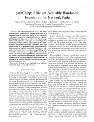
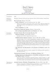
188 Biometrics, March 201320−2(a)0 50 100 150 200 250(b)0.20.100 50 100 150(c)200 25020−20 50 100 150 200 250(d)40−40 50 100 150 200 25010.5(a)00 50 100 150 200 250(b)0.20.100 50 100 150(c)200 25020−20 50 100 150 200 250(d)50−50 50 100 150 200 250Figure 1. Simulated fMRI data with n = 256. Plot (a), first column, refers to the blocked design (period 16), plot (a), secondcolumn, to the event-related design. Plots (b) show a Poisson HRF with λ = 4. Plots (c) show the convolved signal of (a) with(b), and plots (d) the simulated fMRI signal with an I(.2) added noise. Parameters (β,σ 2 ) were set to (.01,1).region and that X B is a basis of neural stimula. A projectionof x R onto the basis is given byx R = X B β, (13)where β is a parameter vector used in expanding x R into X B .Convolution of both sides with an HRF H gives a linear modelwith additive noise of the typey = Xβ + ε, (14)where y = Hx R is an observed fMRI signal at a single voxeland X = HX B is the design matrix representing the convolvedstimulus. Several choices are available for the responsefunction H. Glover (1999) adopted the hemodynamic function(h(t) =c 1 t n 1exp − t )(− a 2 c 2 t n 2exp − t ), (15)t 1 t 2with c 1 =max(t n ie −t/t 2)andwheren 1 =5.0, t 1 =1.1 seconds,n 2 =12.0, t 2 = .9 seconds, and a 2 = .4. Meyer (2003) used thesame HRF as in (15) but with different parameters. Fadili andBullmore (2002) used a Poisson response function with λ =4,h λ (t) = e−λ λ t. (16)t!Residuals of model (14) are typically assumed autocorrelatedand are due to instrumental noise, such as head movementin the scanner. Two types of autocorrelation structureshave been assumed in the literature of fMRI signals:first-order autoregressive and 1/f long memory structures(Smith et al., 1999). A white noise component is sometimesadded to the chosen fMRI noise model, see also our discussionin the Conclusion section. Estimation procedures for fMRItime series with autocorrelated residuals are quite complicatedand computationally expensive. Fadili and Bullmore(2002) applied DWTs and estimated the model parametersin the wavelet domain using an iterative maximum likelihoodestimation method. Meyer (2003) proposed an estimationmethod in the wavelet domain for a generalized linearmodel where a drift is used to explain polynomial trends inthe data. Turkheimer et al. (2003) developed analysis of variance(ANOVA) methods for multiresolution analysis of multisubjectfMRIs. Here we apply our wavelet-based Bayesianapproach, first to simulated fMRI signals and then to realdata. In the real data application we also produce PPMs thataid interpretation by identifying voxels that are likely activatedwith a given confidence.

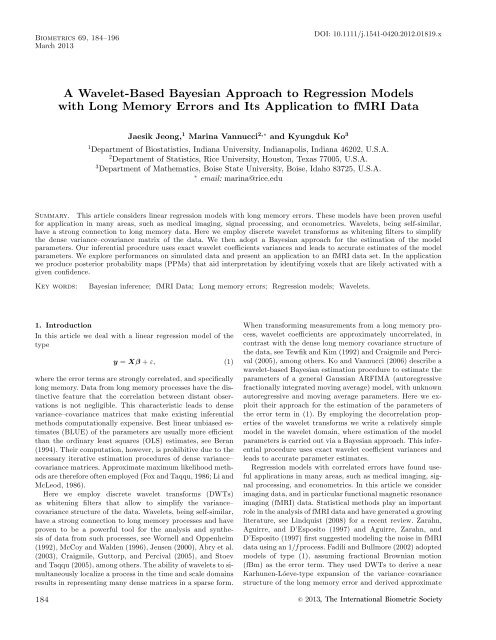
192 Biometrics, March 201310.90.80.70.60.50.40.30.20.1010.90.80.70.60.50.40.30.20.1010.90.80.70.60.50.40.30.20.1010.90.80.70.60.50.40.30.20.1010.90.80.70.60.50.40.30.20.1010.90.80.70.60.50.40.30.20.1010.90.80.70.60.50.40.30.20.1010.90.80.70.60.50.40.30.20.1010.90.80.70.60.50.40.30.20.10Figure 4. fMRI data. Activation maps obtained by mapping probabilities of the estimates of the linear regression parameterβ at each voxel of single slices of image data, thresholded according to the procedure described in the article. First row refersto our method, second row to our implementation of an MLE procedure, and third row to a model with AR(1) noise. Imagesin the first column refer to activations on the primary visual cortex (V1), those in the second column to activations on themotion-selective cortical area (V5), and those in the third column to activations on the posterior parietal cortex (PP).σ 2 had a slight negative bias in almost all cases, indicating underestimation.Also, for fixed N , in most cases the MSEs ofˆd increased as the value of d approached its boundary region(0 or .5). This behavior was also noticed by Jensen (2000), inhis estimation of a model for long memory data contaminatedby white noise, and by Cheung and Diebold (1994). We alsolooked at the results for SNR = 5 and SNR = 10. Table 2 reportsmeans and standard errors for these cases, calculatedover 100 replications. Overall, as expected, we noticed thatthe MSEs were smaller for larger SNR values, that is that thevariability of the estimates decreased as the amplitude of thesignals increased.3.2 Case Study on fMRI DataWe exemplify our method on the epoch data set provided bythe Wellcome Department of Imaging Neuroscience and availableat http://www.fil.ion.ucl.ac.uk/spm/data/. The data setwas originally collected by Büchel and Friston (1997). Belowwe give some description of how the data set was acquiredand refer readers to the original article for more details.• Image Acquisition: The experiment, consisting of fourruns, each lasting 5 minutes 22 seconds, was performedon a single subject using a 2 Telsa Magnetom VISIONwhole body MRI system (Siemens, Erlangen, Germany)equipped with a head volume coil: TE=40 ms, TR=3.22seconds, and 64 × 64 imaging matrix [19.2 × 19.2 cm].Four hundred T ∗ 2 -weighted fMRI images (100 images foreach run) were originally acquired at each of 32 contiguousmultislices (slice thickness 3 mm, giving 9.6 cm verticalfield of view) in the whole brain, except for the lowerhalf of the cerebellum and the most inferior part of thetemporal lobes. The first 10 scans in each run were discardedin order to eliminate magnetic saturation effects.Thus 360 image volumes were used in our estimation procedure.• Experimental Design: The original experiment wasperformed under four different conditions: “Fixation,”“attention,” “no attention,” and “stationary.” The subjectwas asked to look at a fixation point in the middleof a transparent screen. Under visual motion conditions,

Wavelet Approach to Regression Models with Long Memory Errors193250 white dots moved rapidly from the fixation point inrandom directions, at a constant speed, toward the borderof the screen where they vanished. Before scanning,five 30-second trials of the visual stimulus were givenwith five different speeds of the moving dots. During the“attention” and “no attention” conditions the subjectfixated centrally while the white dots emerged from thefixation point toward the edge of the screen. In the “attention”condition the subject was instructed to detectchanges of speed. In the “no attention” condition theinstruction was to just look at the moving points. Duringthe “fixation” condition the subject saw only darkscreen except for the visible fixated dot. In the “stationary”condition the fixation point and 250 stationary dotswere presented to the subject.We applied our wavelet-based Bayesian model to singlevoxels on the 32 contiguous slices. For each voxel we hadN = 360 image volumes. We grouped the four conditions intotwo categories and defined a vector with elements set to 1 forthe images acquired in the “attention” condition and to zerootherwise. We then convolved this vector with the Poissonhemodynamic function with λ = 4 and used the resultingsignal to form the covariate X inmodel(1).Analyseswerecarried out in MATLAB. The estimated parameters weremapped on transverse images using the MRI toolbox 2.0 byDarren Weber.3.2.1 Conditional PPMs. Below we show activations detectedby mapping the estimates of the model parameters ateach voxel of single slices of imaging data and then thresholdingthe corresponding conditional posterior probabilities at aspecified confidence. The resulting PPMs can be seen as amodified version of the posterior maps produced by the softwareSPM following the method of Friston et al. (2002) andFriston and Penny (2003). Our procedure, in particular, isentirely based on the MCMC samples. Let Êβ |y and ˆV β |y bethe mean and variance of a realization of β from the Markovchain at a single voxel. We define the resulting conditionalposterior probability p for that voxel as⎛ ⎞p =1− Φ ⎝ κ − Êβ |y√ ⎠ , (19)ˆV β |ywhere Φ is the standard normal distribution function and κis the thresholding rule set asκ = ζ + z α√ˆV β |y , (20)with ζ the standard deviation of Ê β |y over all voxels in theslice, which we estimate based on the MCMC samples as thestandard deviation of the posterior estimates of β over allvoxels, and z α the upper α percentile of the standard normaldistribution. In the applications we set α to .05, that is,we used z α =1.64, to obtain activation maps thresholded ata 95% confidence. In the PPM of Friston et al. (2002) andFriston and Penny (2003), the posterior mean and variance ofβ are used instead of Êβ |y and ˆV β |y , respectively, and ζ in (20)is estimated from the prior. One should be careful when interpretingthe maps obtained by thresholded conditional posteriorprobabilities. In particular, a voxel showing a high valuedoes not indicate activation but rather a high chance of beingactivated. This aids interpretation as one can easily identifythe voxels with posterior chances for being activated with agiven confidence.3.2.2 Results. In analyzing fMRI data we followed the approachof Wornell and Oppenheim (1992) and McCoy andWalden (1996) and assumed a variance progression formulafor the wavelet coefficients of the typeσ 2 σ 2 mn = σ 2 (2 α ) −m , (21)with α ∈ (0, 1) the long memory parameter and σ 2 the innovationvariance. The reason for this choice is that it resultsin an error term, which is not restricted to a specific class oflong memory processes, like I(d), but rather it encompassesthe general fractal process of type (2), including long memoryprocesses. In particular, we are not restricting the long memoryparameter to the stationary range, as it is instead in thecase of I(d) processes (Long et al., 2005). For inference, weused a very similar MCMC procedure to what described inSection 2.4, with Gibbs’s steps for β and σ 2 and a Metropolisstep on α with a Gaussian proposal centered in the previousvalue and a standard deviation of .05, which worked well forus.Neuroimaging studies have shown that a stimulus with visualmotion, like the rapidly moving dots in this experiment,activates the primary visual cortex, the motion-selective corticalarea, and the posterior parietal cortex, see Bushnell,Goldberg, and Robinson (1981), Mountcastle, Anderson, andMotter (1981), and Treue and Maunsell (1996). We thereforefocused on these regions. Figure 3 shows activations maps obtainedby mapping the estimates of the regression parameterβ (first row), the innovation variance σ 2 (second row), andthe long memory parameter α (third row), at each voxel ofsingle slices of image data, obtained with our method. Imagesin the first column refer to activations on the primaryvisual cortex (V1; 2275 voxels), those in the second columnto activations on the motion-selective cortical area (V5; 2327voxels), and those in the third column to activations on theposterior parietal cortex (PP; 1325 voxels). Brighter colorson the images denote higher estimated values of the parameter,that is stronger activations (or cerebral responses) to thegiven visual stimulus.In Figure 4 we compare the activation maps obtained bymapping probabilities of the estimates of the linear regressionparameter β, as described earlier, with equivalent maps obtainedwith two competing methods: an MLE method (secondrow), which we implemented as described in the Appendix,and a model with an AR(1) noise (third row) that ignores thelong-memory nature of the data. Columns refer to the V1, V5,and PP regions, respectively. Brighter colors on the images denotehigh chance of strong activations (or cerebral responses)to the given visual stimulus. The areas most likely activatedby the given “attentional” visual stimulus correspond to thespatial coordinates of the V1, V5, and PP areas of the subject,as identified by Büchel and Friston (1997). All methodscorrectly detect activations in the designated areas, with activationsthat occur quite broadly around the corresponding

194 Biometrics, March 2013coordinates of V1, V5, and PP. Notice, however, that the detectionis much sharper with our Bayesian maps.Other authors have compared estimation performances ofmodels for fMRI data that make different assumptions on theerror structure and have pointed out that models ignoringthe long memory autocorrelation in the errors result in standarderrors of the estimates that are inflated, see for example,Friston and Penny (2003). Our maps in Figure 3 confirm thatfMRI data are indeed contaminated by long memory errorsand that some of the cerebral responses have large values ofα. Also, they show that the innovation variance of the longmemory error is not uniformly distributed over the brain andthat it has relatively large values in very small parts aroundthe center area and in outer area of the brain. Several authorshave pointed out that fMRI signals are contaminated by instrumentaland physiological noises. The sources for such errorsare, however, not completely known. Long memory noise,in particular, has been attributed to head movement causedby slow rotation or translation during scanning, as well as tocardiac and respiratory cycle-related pulsations. Neurophysiologicalsources could be hypothesized too. However, it is stillan open question whether fMRI noise may indeed reveal informationon brain activity, such as long-range dependenciesin response to stimula.4. ConclusionsIn this article we have proposed a wavelet-based method toestimate the parameters of a regression model with an 1/f errorcomponent. We have carried out estimation in the waveletdomain in order to simplify the treatment of the dense covariancematrix of the long memory error, and have used aBayesian approach for the estimation of the model parameters.Our inferential procedure uses exact wavelet coefficientsvariances and leads to accurate estimates of the model parameters.Although we have chosen to mainly focus on the fractionallyintegrated long memory processes of Hosking (1981)and Granger and Joyeux (1980), our inferential procedurecan be easily extended to handle more general classes of longmemory processes. For example, in the application of this articlewe have employed a very general variance progressionformulation. Whitening properties of DWTs for long memoryprocesses are well documented (Tewfik and Kim, 1992;Craigmile and Percival, 2005; Ko and Vannucci, 2006, amongothers). Furthermore, wavelet packets have been investigatedas a more general tool that can decorrelate other processesthan the long memory, see Percival, Sardy, and Davison (2001)and Gabbanini et al. (2004).We have evaluated performances of our method on simulateddata and also showed an application to fMRI data.Results have confirmed that our wavelet-based approach issuitable for applications to fMRI data. There we have producedPPMs that aid interpretation, as one can easily identifyvoxels that are likely activated with a given confidence.Single-subject scanning is receiving renewed interest in thefMRI field, due to its use for presurgical purposes. In addition,our approach can be used to produce single-subjectposterior maps as a form of meta-analysis for intersubject investigations,similarly in spirit to other Bayesian approachesto fMRI modeling (Bowman et al., 2008).As a possible extension of the model we have presented, ina basic study on the analysis of fMRI time series (Zarahnet al., 1997) argue that fMRI signals are contaminatedby a white noise in addition to long memory noise, andWornell and Oppenheim (1992) develop an estimation procedureof the model parameters under two additive noises.Other interesting extensions include models accounting forthe estimation of the HRF and/or Bayesian spatiotemporalmodels that incorporate spatial correlation among brain responsesvia network priors (Gossl, Auer, and Fahrmeir, 2001;Quiros, Montes-Diez, and Gamerman, 2010).5. Supplementary MaterialsMatlab code and fMRI data are available with this article atthe Biometrics website on Wiley Online Library.AcknowledgementVannucci is partially supported by NSF/DMS grant DMS-1007871.ReferencesAbry, P., Flandrin, P., Taqqu, M. S., and Veitch, D. (2003).Self-similarity and long-range dependence through the waveletlens. In Theory and Applications of Longrange Dependence, P.Doukhan, G. Oppenheim, and M. Taqqu (eds), 526–556. Boston:Birkhauser.Aguirre, G., Zarahn, E., and D’Esposito, M. (1997). Empirical analysesof BOLD fMRI statistics II. NeuroImage 5, 199–212.Beran, J. (1994). Statistics for Long-Memory Processes. New York:Chapman & Hall.Bowman, F., Caffo, B., Bassett, S., and Kilts, C. (2008). Bayesian hierarchicalframework for spatial modeling of fMRI data. NeuroImage39, 146–156.Büchel, C. and Friston, K. (1997). Modulation of connectivity in visualpathways by attention: Cortical interactions evaluated withstructural equation modelling and fMRI. Cerebral Cortex 7,768–778.Bullmore, E., Fadili, J., Maxim, V., Sendur, L., Whitcher, B., Suckling,J., Brammer, M., and Breakspear, M. (2004). Wavelets andfunctional magnetic resonance imaging of the human brain. NeuroImage23, 234–249.Bushnell, M., Goldberg, M., and Robinson, D. (1981). Behavioral enhancementof visual responses in monkey cerebral in monkeycerebral cortex. I. Modulation in posterior parietal cortex relatedto selective visual attention. Journal of Neurophysiology 46,755–772.Buxton, R. and Frank, L. (1997). A model for the coupling betweencerebral blood flow and oxygenation metabolism during neuralstimulation. Journal of Cerebral Blood Flow Metabolism 17,64–72.Cheung, Y. and Diebold, F. (1994). On maximum likelihood estimationof the differencing parameter of fractionally-integrated noise withunknown mean. Journal of Econometrics 62, 301–306.Craigmile, P., Guttorp, P., and Percival, D. (2005). Wavelet-based parameterestimation for polynomial contaminated fractionally differencedprocesses. IEEE Transactions on Signal Processing 53,3151–3161.Craigmile, P. F. and Percival, D. B. (2005). Asymptotic decorrelationof between-scale wavelet coefficients. The IEEE Transactions onInformation Theory 51, 1039–1048.

Wavelet Approach to Regression Models with Long Memory Errors195Daubechies, I. (1992). Ten Lectures on Wavelets, Volume 61: CBMS-NSF Conference Series. SIAM.Fadili, M. and Bullmore, E. (2002). Wavelet-generalised least squares:A new BLU estimator of linear regression models with 1/f errors.NeuroImage 15, 217–232.Fox, R. and Taqqu, M. (1986). Large-sample properties of parameterestimates for strongly dependent stationary Gaussian time series.Annals of Statistics 14, 517–532.Friston, K., Holmes, A., Price, C., Buchel, C., and Worsley, K. (1999).Multisubject fMRI studies and conjunction analyses. NeuroImage10, 385–396.Friston, K. and Penny, W. (2003). Posterior probability maps andSPMs. NeuroImage 19, 1240–1249.Friston, K., Penny, W., Phillips, C., Kiebel, S., Hinton, G., andAshburner, J. (2002). Classical and Bayesian inference in neuroimaging:Theory. NeuroImage 16, 465–483.Gabbanini, F., Vannucci, M., Bartoli, G., and Moro, A. (2004). Waveletpacket methods for the analysis of variance of time series withapplication to crack widths on the Brunelleschi dome. Journal ofComputational and Graphical Statistics 13, 639–658.Geweke, J. and Porter-Hudak, S. (1983). The estimation and applicationof long memory time series models. Journal of Time SeriesAnalysis 4, 221–237.Glover, G. (1999). Deconvolution of impulse response in event-relatedBOLD fMRI. NeuroImage 9, 416–429.Gossl, C., Auer, D., and Fahrmeir, L. (2001). Bayesian modeling of thehemodynamic response function in BOLD fMRI. Neuroimage 14,140–148.Granger, C. and Joyeux, R. (1980). An introduction to long memorytime series models and fractional differencing. Journal of TimeSeries Analysis 1, 15–29.Guo, Y., Bowman, F., and Kilts, C. (2008). Predicting the brain responseto treatment using a Bayesian hierarchical model withapplication to a study of schizophrenia. Human Brain Mapping29, 1092–1109.Haslett, J. and Raftery, A. (1989). Space-time modeling with longmemorydependence: Assessing Ireland’s wind power resource.Journal of Applied Statistics 38, 1–50.Hosking, J. (1981). Fractional differencing. Biometrika 68, 165–176.Jensen, M. (2000). An alternative maximum likelihood estimatorof long-memory processes using compactly supported wavelets.Journal of Economic Dynamics and Control 24, 361–386.Ko, K. and Vannucci, M. (2006). Bayesian wavelet analysis of autoregressivefractionally integrated moving-average processes. Journalof Statistical Planning and Inference 136, 3415–3434.Li, W. and McLeod, A. (1986). Fractional time series modelling.Biometrika 73, 217–221.Lindquist, M. (2008). The statistical analysis of fMRI data. StatisticalScience 23, 439–464.Long, C., Brown, E., Triantagfyllou, C., Aharon, I., Wald, L., and Solo,V. (2005). Nonstationary noise estimation in functional MRI.NeuroImage 28, 890–903.Mallat, S. (1989). A theory for multiresolution signal decomposition:The wavelet representation. IEEE Transactions on Pattern Analysisand Machine Intelligence 11, 674–693.McCoy, E. and Walden, A. (1996). Wavelet analysis and synthesis ofstationary long-memory processes. Journal of Computational andGraphical Statistics 5, 26–56.McLeod, A. and Hipel, K. (1978). Preservation of the rescaled adjustedrange. Parts 1, 2 and 3. Water Resources Research 14,491–512.Meyer, F. (2003). Wavelet-based estimation of a semiparametric generalizedlinear model of fMRI time-series. IEEE Transactions onMedical Imaging 22, 315–322.Mountcastle, V., Anderson, R., and Motter, B. (1981). The influenceof attentive fixation upon the excitability of the light-sensitiveneurons of the posterior parietal cortex. Journal of Neuroscience1, 1218–1225.Percival, D., Sardy, S., and Davison, A. (2001). Wavestrapping time series:Adaptive wavelet-based bootstraping. In Nonlinear and NonstationarySignal Processing, W. Fitzgerald, R. Smith, A. Walden,and P. Young (eds). Cambridge, England: Cambridge UniversityPress.Quiros, A., Montes-Diez, R., and Gamerman, D. (2010). Bayesian spatiotemporal model of fMRI data. NeuroImage 49, 442–456.Smith, A., Lewis, B., Ruttimann, U., Ye, F., Sinwell, T., Yang,Y., Duyn, J., and Frank, J. (1999). Investigation of low frequencydrift in fMRI signals. NeuroImage 9, 526–533.Stoev, S. and Taqqu, M. S. (2005). Asymptotic self-similarity andwavelet estimation for long-range dependent fractional autoregressiveintegrated moving average time series with stable innovations.Journal of Time Series Analysis 26, 211–249.Taswell, C. and McGill, K. (1994). Wavelet transform algorithms forfinite-duration discrete-time signals. ACM Transactions on MathematicalSoftware 20, 398–412.Tewfik, A. and Kim, M. (1992). Correlation structure of the discretewavelet coefficients of fractional Brownian motion. IEEE Transactionson Information Theory 38, 904–909.Tie, Y., Suarez, R., Whalen, S., Radmanesh, A., Nortan, I., andGolby, A. (2009). Comparison of blocked and event-relatedfMRI designs for pre-surgical language mapping. NeuroImage 47,T107–T115.Treue, S. and Maunsell, H. (1996). Attentional modulation of visualmotion processing in cortical areas MT and MST. Nature 382,539–541.Turkheimer, F., Aston, J., Banati, R., Riddle, C., and Cunningham,V. (2003). A linear wavelet filter for parametric imagingwith dynamic. IEEE Transactions on Medical Imaging 22,289–301.Vannucci, M. and Corradi, F. (1999). Covariance structure of waveletcoefficients: Theory and models in a Bayesian perspective. Journalof the Royal Statistical Society, Series B 61, 971–986.Woolrich, M., Jenkinson, M., Brady, J., and Smith, S. (2004). FullyBayesian spatio-temporal modeling of fMRI data. IEEE Transactionson Medical Imaging 23, 213–231.Wornell, G. and Oppenheim, A. (1992). Estimation of fractal signalsfrom noisy measurements using wavelets. IEEE Transactions onSignal Processing 40, 611–623.Zarahn, E., Aguirre, G., and D’Esposito, M. (1997). Empirical analysesof BOLD fMRI statistics I. NeuroImage 5, 179–197.Received October 2011. Revised July 2012.Accepted July 2012.AppendixDerivation of the MLE of Θ =(β,σ 2 ,η)The likelihood function of model (10) with one explanatoryvariable X w isL(Θ) = (σ2 ) −N/2 |Σ Ψ | −1/ 2( √ exp2π)[N× − 1]2σ (y 2 w − X w β) ′ Σ −1Ψ (y w − X w β) ,where Σ Ψ is a diagonal matrix whose elements are(2 α ) −m ,m =1,...,r. We consider only one explanatory variable,but the derivation can be easily extended to multipleexplanatory variables. Let η =2 α in the variance progression

196 Biometrics, March 2013(21). Maximizing L(Θ), we have the following maximum likelihoodestimates of Θ:r∑ˆη =argmax η T m K m η m ,where∑ N (m )n =1ˆσ 2 =m =1r∑K m ˆη / ∑rm N (m),m =1m =1∑ N (m )ˆη m yn =1 m,nX m,n∑r ∑ N (m )ˆη m X 2 m =1 n =1m,nˆβ =∑ rm =1T m = ∑ rmN(m) − m ∑ rN (m) and K m =1 m =1 m =(y m,n − βX m,n ) 2 . The estimates ˆη and ˆσ 2 follow fromWornell and Oppenheim (1992) via the normal equations,r∑r∑N (m) = η m K m ,σ 2m =1m =1,r∑mN(m) =σ −2m =1r∑mη m K m .m =1Figure 4 shows activation maps obtained by mapping probabilitiesof the estimates of the linear regression parameter βat each voxel of a single slice obtained with the method describedearlier. To obtain these maps, we applied a thresholdingrule similar to the one we employ in our Bayesian estimationmethod, that is,( )ϑ −p =1− Φ √ ˆβ , ˆV (β)where ϑ is set to ϑ = Ê(β)+z α√ ˆV (β)with Ê(β)and√ ˆV (β)the mean and standard deviation of the estimated β’s over allvoxels in the slice. Here ˆβ denotes the estimate of β at eachvoxel. We set α = 05, that is, z α =1.64.