slides in pdf format - Department of Statistics - Rice University

Using Population Structure to Map Complex
Diseases
Bo Peng † (bpeng@rice.edu)
Dr. William Amos ‡ (w.amos@zoo.cam.ac.uk)
Dr. Marek Kimmel † (kimmel@rice.edu)
† Department of Statistics, Rice University
‡ Department of Zoology, University of Cambridge
July, 2004
Keck Fellows Meeting, July 2004

Outline
1. Background ideas
• Genetic diseases and population structure
• Problems of current approaches, and
• How some new ideas might help

Outline
1. Background ideas
• Genetic diseases and population structure
• Problems of current approaches, and
• How some new ideas might help
2. Some tech details
• Basics of relatedness and inbreeding coefficient
• How to estimate relatedness using genetic marker data

Outline
1. Background ideas
• Genetic diseases and population structure
• Problems of current approaches, and
• How some new ideas might help
2. Some tech details
• Basics of relatedness and inbreeding coefficient
• How to estimate relatedness using genetic marker data
3. An example
Keck Fellows Meeting, July 2004 1

Genetic diseases
A genetic disease is a disease caused by abnormalities in an individuals’ genetic
material (genome).
A simple disease (e.g. cystic fibrosis) is caused by a defect in only one gene.
By contract, complex diseases (e.g. most cancers) are caused by many variations
occurred in different genes in the same cell. Different variations may lead to the
same symptoms.

Genetic diseases
A genetic disease is a disease caused by abnormalities in an individuals’ genetic
material (genome).
A simple disease (e.g. cystic fibrosis) is caused by a defect in only one gene.
By contract, complex diseases (e.g. most cancers) are caused by many variations
occurred in different genes in the same cell. Different variations may lead to the
same symptoms.
It is of vast interest to find out which gene(s) are responsible for a genetic
disease. This is in general called gene mapping. Many methods have been developed
but the results have been disappointing compared to the money invested.
• There are some success in mapping simple disease like cystic fibrosis, but not
many.
• Very few genes have been found for complex diseases.
• Amont these genes, only a small fraction of them (∼ 5% ) can be consistently
replicated by other researchers.

Genetic diseases
A genetic disease is a disease caused by abnormalities in an individuals’ genetic
material (genome).
A simple disease (e.g. cystic fibrosis) is caused by a defect in only one gene.
By contract, complex diseases (e.g. most cancers) are caused by many variations
occurred in different genes in the same cell. Different variations may lead to the
same symptoms.
It is of vast interest to find out which gene(s) are responsible for a genetic
disease. This is in general called gene mapping. Many methods have been developed
but the results have been disappointing compared to the money invested.
• There are some success in mapping simple disease like cystic fibrosis, but not
many.
• Very few genes have been found for complex diseases.
• Amont these genes, only a small fraction of them (∼ 5% ) can be consistently
replicated by other researchers.
Keck Fellows Meeting, July 2004 2

Life of a disease gene – a hard one
Genetic diseases are introduced by mutation and spread through mating.

Life of a disease gene – a hard one
Genetic diseases are introduced by mutation and spread through mating.
• Every allele is subject to a random sampling process if it is to survive to the next
generation. The process is called genetic drift. Because the chance of survival
of an allele is proportional to its frequency in population, most newborns (new
mutations) get lost quickly because of genetic drift.

Life of a disease gene – a hard one
Genetic diseases are introduced by mutation and spread through mating.
• Every allele is subject to a random sampling process if it is to survive to the next
generation. The process is called genetic drift. Because the chance of survival
of an allele is proportional to its frequency in population, most newborns (new
mutations) get lost quickly because of genetic drift.
• The hosts of disease alleles usually have smaller chance to produce offspring
(selective disadvantage). Many disease genes are thus eliminated by selection.

Life of a disease gene – a hard one
Genetic diseases are introduced by mutation and spread through mating.
• Every allele is subject to a random sampling process if it is to survive to the next
generation. The process is called genetic drift. Because the chance of survival
of an allele is proportional to its frequency in population, most newborns (new
mutations) get lost quickly because of genetic drift.
• The hosts of disease alleles usually have smaller chance to produce offspring
(selective disadvantage). Many disease genes are thus eliminated by selection.
• Mating is usually regional so traveling (migration) is not easy, especially in the
old days.
Keck Fellows Meeting, July 2004 3

Life of a disease gene – some good news
• New alleles can be generated by recurrent mutation. However, this is usually
not the case since almost all mutations are unique. Instead, new mutations may
lead to the same or slightly different phenotypes (disease).

Life of a disease gene – some good news
• New alleles can be generated by recurrent mutation. However, this is usually
not the case since almost all mutations are unique. Instead, new mutations may
lead to the same or slightly different phenotypes (disease).
• There are late-onset diseases (such as Alzheimer’s disease) that do not affect
reproduction. So selection is almost neutral in these cases.

Life of a disease gene – some good news
• New alleles can be generated by recurrent mutation. However, this is usually
not the case since almost all mutations are unique. Instead, new mutations may
lead to the same or slightly different phenotypes (disease).
• There are late-onset diseases (such as Alzheimer’s disease) that do not affect
reproduction. So selection is almost neutral in these cases.
• Heterozygous disease allele carriers may have some selective advantages (heterozygous
advantage) that helps the survival of disease allele.

Life of a disease gene – some good news
• New alleles can be generated by recurrent mutation. However, this is usually
not the case since almost all mutations are unique. Instead, new mutations may
lead to the same or slightly different phenotypes (disease).
• There are late-onset diseases (such as Alzheimer’s disease) that do not affect
reproduction. So selection is almost neutral in these cases.
• Heterozygous disease allele carriers may have some selective advantages (heterozygous
advantage) that helps the survival of disease allele.
• A disease gene may get fixed (becomes the only allele at the locus) and live
happily ever after. This happens much easier in small subpopulations with
non-random mating.

Life of a disease gene – some good news
• New alleles can be generated by recurrent mutation. However, this is usually
not the case since almost all mutations are unique. Instead, new mutations may
lead to the same or slightly different phenotypes (disease).
• There are late-onset diseases (such as Alzheimer’s disease) that do not affect
reproduction. So selection is almost neutral in these cases.
• Heterozygous disease allele carriers may have some selective advantages (heterozygous
advantage) that helps the survival of disease allele.
• A disease gene may get fixed (becomes the only allele at the locus) and live
happily ever after. This happens much easier in small subpopulations with
non-random mating.
• Migration is getting easier!
Keck Fellows Meeting, July 2004 4

What do all these tell us
• Disease gene tends to form clusters among spatially and/or genetically
related individuals/families. Even among affected individuals/families, we
may still expect clustering of disease alleles within the population. ( Illustration:
spatial distribution of alleles )

What do all these tell us
• Disease gene tends to form clusters among spatially and/or genetically
related individuals/families. Even among affected individuals/families, we
may still expect clustering of disease alleles within the population. ( Illustration:
spatial distribution of alleles )
• Many diseases are recessive. Disease alleles are more likely to be expressed
in individuals born to related parents, and in particular to parents who are
closely related for the section of their genome in which a susceptibility factor
lies. Consequently, the presence of recessive factors can be inferred wherever
affected individuals exhibit unusually elevated levels of relatedness
between homologous chromosomes at some place in their genome. (
Illustration: homologous chromosomes )
Keck Fellows Meeting, July 2004 5

Basic gene mapping methods
Genes that are close to a disease gene tend to co-segregate with it during
meiosis. Therefore, if a gene is over/under-present in the diseased population than
in the general population, this gene might be close to one of the disease genes.

Basic gene mapping methods
Genes that are close to a disease gene tend to co-segregate with it during
meiosis. Therefore, if a gene is over/under-present in the diseased population than
in the general population, this gene might be close to one of the disease genes.
This leads to case-control studies:
• Collect two groups of people, one with disease (case group) and one without
(control group).
• Find out the genotypic information of as many markers as funding allows, and
compare the allele frequencies of case and control groups.
If the population is genetically homogeneous and the marker is not linked to a
susceptibility factor (disease locus), these allele frequencies should roughly be the
same. Any significant difference in allele frequency can then be used to infer an
association (linkage) between the marker and a disease locus.
Keck Fellows Meeting, July 2004 6

What trouble can population structure make
The homogeneity assumption does not hold in the presence of population
structure, when both disease frequency and marker allele frequencies can differ
among subpopulations.

What trouble can population structure make
The homogeneity assumption does not hold in the presence of population
structure, when both disease frequency and marker allele frequencies can differ
among subpopulations.
For example: suppose a sample of cases and controls is drawn from a population
containing a number of subpopulations. If the disease of interest is at high frequency
in one subpopulation, then we can expect to find that group overrepresented among
the cases. Then, any marker allele that is at higher frequency in that subpopulation
than in the others will appear to be associated with the disease, regardless of where
it is in the genome. In other words, a spurious association will be found.
Keck Fellows Meeting, July 2004 7

In the case of complex disease
Population structure is more important when mapping complex diseases because
• Disease susceptibility factors are likely to contribute to some families but not to
others;
• Disease gene tends to form clusters among spatially and/or genetically related
individuals/families.
If we treat families as independent observations, families for whom the factor is not
important or present will contribute background noise that may mask the signal
from those families where it does play a role.
Keck Fellows Meeting, July 2004 8

Current Fixes to Population Structure
Population admixture has been widely recognized as the major reason for
nonreplicability associations [Ardie et al 2002 ]. To overcome this problem, people either
avoid population based case control studies ( use TDT tests instead ) or
• use markers throughout the genome to adjust for any inflation in test statistics
due to substructure ( Genomic control [Bacanu et al 2000, Devlin et al 2001] )
• infer the details of the subpopulations ( Structured Association [ Pritchard et al 2000,
Thornsberry et al 2001 ], etc)
However, there are no clear-cut subpopulations in a sample in many cases. Even
there are, it is very difficult to estimate the number of subpopulations and classify
samples into them. Homogeneity within subpopulations is also hard to prove.
Keck Fellows Meeting, July 2004 9

Using Population Structure to Map Complex Diseases
We have developed an algorithm to map complex diseases. We do not explicitly
identify subpopulations. Instead, we construct a neighborhood of families for each
family by putting weights on families according to family relatedness measures.

Using Population Structure to Map Complex Diseases
We have developed an algorithm to map complex diseases. We do not explicitly
identify subpopulations. Instead, we construct a neighborhood of families for each
family by putting weights on families according to family relatedness measures.
• Estimate family relatedness using marker data. The family relatedness
measures are the averaged relatedness coef between all inter-family offspring
combinations, which can be estimated by, for example, Queller’s Method [ Queller
1989, Lynch et al 1999 ]
ˆr xy =
1
2 (δ ac + δ ad + δ bc + δ bd ) − p a − p b
1 + δ ab − p a − p b
where (a, b), (c, d) are genotypes of individual x and y. p a is the population
frequency of allele a.
• Define a weighting system that falls off with increasing distance away along
the chromosome and also with decreasing relatedness across families.
Keck Fellows Meeting, July 2004 10

Our Approach (cont.)
• Measure the inbreeding level of each locus for each family. The locus-level
inbreeding measures are estimated by, for example, Internal Relatedness
ˆr x = 2δ ab − p a − p b
2 − p a − p b
• Average the inbreeding measures using the
weighting system. We infer the presence of
recessive factors wherever affected individuals exhibit
unusually elevated levels of relatedness between
homologous chromosomes at some place in
their genome.
• The significance of high average measures can be tested by randomizing
the relatedness values and the marker locations and asking the extent to which
the observed sum is large relative to randomized measures.
Keck Fellows Meeting, July 2004 11

Tech details: Inbreeding Coefficient
Inbreeding means mating between closely related individuals. (Illustration:
inbreeding) Inbreeding Coefficient is the probability that random alleles in different
individuals/groups have descended from a single ancestral allele (this is called ibd:
Identical by descent)

Tech details: Inbreeding Coefficient
Inbreeding means mating between closely related individuals. (Illustration:
inbreeding) Inbreeding Coefficient is the probability that random alleles in different
individuals/groups have descended from a single ancestral allele (this is called ibd:
Identical by descent) Note that
• Relatedness between two individuals/groups with multiple loci are the average
of locus level relatedness measures.

Tech details: Inbreeding Coefficient
Inbreeding means mating between closely related individuals. (Illustration:
inbreeding) Inbreeding Coefficient is the probability that random alleles in different
individuals/groups have descended from a single ancestral allele (this is called ibd:
Identical by descent) Note that
• Relatedness between two individuals/groups with multiple loci are the average
of locus level relatedness measures.
• This concept can be generalized to inbreeding of one individual or one population.
In these cases, ‘random alleles’ are picked from an individual (with two alleles)
or a group of individuals (random alleles from random individuals within this
group).

Tech details: Inbreeding Coefficient
Inbreeding means mating between closely related individuals. (Illustration:
inbreeding) Inbreeding Coefficient is the probability that random alleles in different
individuals/groups have descended from a single ancestral allele (this is called ibd:
Identical by descent) Note that
• Relatedness between two individuals/groups with multiple loci are the average
of locus level relatedness measures.
• This concept can be generalized to inbreeding of one individual or one population.
In these cases, ‘random alleles’ are picked from an individual (with two alleles)
or a group of individuals (random alleles from random individuals within this
group).
• Inbreeding coefficient has other names such as coefficient of coancestry, Consanguinity
coefficient, Kinship. They commonly refer to inbreeding between two
individuals.
Keck Fellows Meeting, July 2004 12

Population Explanation of Inbreeding Coefficient
Suppose that p and q are frequency of two alleles at a locus. Under HWE, the
frequency of heterozygous genotype should be 2pq, we call this frequency in general
H 0 . In case of breeding, this frequency is H 1 and inbreeding coefficient (for this
population)F is defined as
F = H 0 − H 1
H 0
One can deduce formulae of genotype frequencies in a population with inbreeding
level F . We can see that inbreeding causes a decrease of heterozygosity.
genotype frequency wih inbreeding under Hardy-Weinberg Equilibrium
AA p 2 + pqF p 2
Aa 2pq (1 − F ) 2pq
aa q 2 + pqF q 2
Keck Fellows Meeting, July 2004 13

Estimate Inbreeding Coef. from Pedigree Data
Wright’s (1922) formula:
F I = ∑ i
( 1
2
) ni
(1 + F Ai )
where i is the ith common ancestor, n i is
the number of individuals inside the loop
I → A i → I.

Estimate Inbreeding Coef. from Pedigree Data
Wright’s (1922) formula:
F I = ∑ i
( 1
2
) ni
(1 + F Ai )
where i is the ith common ancestor, n i is
the number of individuals inside the loop
I → A i → I.
For the left pedigree, n G = 2,
F I =
( 1
2
) 2
(1 + F G ) = 1 4
Keck Fellows Meeting, July 2004 14

Family Level Relatedness: Dr. Queller’s Method
Pedigree data is usually unavailable between families. (Need huge pedigrees)
Fortunately, progress in the developing of methods of estimating parental relatedness
from marker data has been rapid. Suppose that individuals x has genotype (a, b)
and individual y has genotype . Suppose that the allele frequencies of these alleles
are p a , p b , p c , p d . The (directional) relatedness between x and y is given by
ˆr xy =
1
2 (δ ac + δ ad + δ bc + δ bd ) − p a − p b
1 + δ ab − p a − p b
where δ ac = 1 if a = c and 0 otherwise. Usually, directional measures are averaged
to get a better estimate, the formula becomes
ˆr xy = δ ac + δ ad + δ bc + δ bd − p a − p b − p c − p d
2 + δ ab + δ cd − p a − p b − p c − p dd
Keck Fellows Meeting, July 2004 15

Dr. Queller’s Method (Cont. 1)
• When multiple markers are available, the relatedness measure is the average of
locus-level measures.

Dr. Queller’s Method (Cont. 1)
• When multiple markers are available, the relatedness measure is the average of
locus-level measures.
• Relatedness measures between two groups is the average of relatedness coef
between all inter-family offspring combinations.

Dr. Queller’s Method (Cont. 1)
• When multiple markers are available, the relatedness measure is the average of
locus-level measures.
• Relatedness measures between two groups is the average of relatedness coef
between all inter-family offspring combinations.
• Simulation results indicate that a+b
c+d averaging performs better than 1 2
( a
c + b d)
.
It is therefore preferable to keep track of numerator/denominator at all time
during calculation.

Dr. Queller’s Method (Cont. 1)
• When multiple markers are available, the relatedness measure is the average of
locus-level measures.
• Relatedness measures between two groups is the average of relatedness coef
between all inter-family offspring combinations.
• Simulation results indicate that a+b
c+d averaging performs better than 1 2
( a
c + b d)
.
It is therefore preferable to keep track of numerator/denominator at all time
during calculation.
• Other methods are also available, notable from Lynch 1999.
Keck Fellows Meeting, July 2004 16

Locus Level Relatedness Measures
The following measures have been proposed:
• Heterozygosity (Het)
Straight heterozygosity does uncover strong effects in natural populations of
animals and plants, but remains a somewhat crude measure.

Locus Level Relatedness Measures
The following measures have been proposed:
• Heterozygosity (Het)
Straight heterozygosity does uncover strong effects in natural populations of
animals and plants, but remains a somewhat crude measure.
• d-squared (d 2 )
Microsatellite alleles diverge in a way such that the square of the length difference
between a pair of alleles may be linearly related to time since their common
ancestor. Consequently, the average squared allele length difference across either
loci or individuals provides an estimator for overall genomic similarity. Let
Mx (h) be the number of alleles at locus h, denote the genotype of individual
i as (a ih , b ih ),
d 2 = mean
( ) 2
aih − b ih
Mx (h) − 2
Keck Fellows Meeting, July 2004 17

Locus Level Relatedness Measure (Cont.)
• Standardized heterozygosity (SH) and Standardized Observed Heterozygosity
(SOH)
SH is heterozygosity but weighted by the expected heterozygosity at each locus
scored. SOH is a version of SH where the correction is made using observed
heterozygosity, rather than expected heterozygosity. This is a more robust
method in comparison with others.

Locus Level Relatedness Measure (Cont.)
• Standardized heterozygosity (SH) and Standardized Observed Heterozygosity
(SOH)
SH is heterozygosity but weighted by the expected heterozygosity at each locus
scored. SOH is a version of SH where the correction is made using observed
heterozygosity, rather than expected heterozygosity. This is a more robust
method in comparison with others.
• Internal Relatedness
Internal relatedness was developed by William Amos in Cambridge and quantifies
the degree of heterozygosity weighted by the frequencies of the alleles in each
genotype. Using the similar notation as that of d 2 measure
IR =
∑ ∑
i
h
∑
i
(
2δaih =b ih
− f aih − f bih
)
∑ ( )
h 2 − faih − f bih
Keck Fellows Meeting, July 2004 18

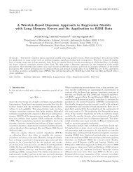
Log P-values of Locus Association
Leprosy dataset
[Siddiqui et al 2001]
394 individuals
96 nuclear
families
all offsprings are
affected
295 microsatellite
markers on 22
autosomes are
typed
0 1 2 3 4 5
25
D10S591
7
D10S189
18
D10S547
9
D10S191
1
D10S1653
5
D10S1763
3
D10S1661
19
D10S548
4
D10S1662
Overall Measures on Chromosome 10
22
D10S582
23
D10S586
20
D10S563
2
D10S1660
loci
21
D10S572
11
D10S197
13
D10S208
16
D10S220
0
D10S1652
17
D10S537
12
D10S201
6
D10S185
10
D10S192
8
D10S190
24
D10S587
15
−log(P−value)
scaled IBD MLS
AfIR
UnIR
AfRel
D10S217
14
D10S212
Our result confirms the reported susceptibility locus on chromosome 10, as well
as most of the less-significant ones.
Keck Fellows Meeting, July 2004 19

• What I have done
Summary and Future Work
⋆ Implement a fast (relative to the extensive computation needed) and flexible
algorithm that can perform our method using various family level and locus
level relatedness measures, and various randomization methods;
⋆ Test our algorithm on six real datasets; Test the robustness of our algorithm
using partial information of the datasets;
⋆ Compare the performance of two family-level relatedness measures;
⋆ Present a poster at the 9th Structural Biology Symposium.

• What I have done
Summary and Future Work
⋆ Implement a fast (relative to the extensive computation needed) and flexible
algorithm that can perform our method using various family level and locus
level relatedness measures, and various randomization methods;
⋆ Test our algorithm on six real datasets; Test the robustness of our algorithm
using partial information of the datasets;
⋆ Compare the performance of two family-level relatedness measures;
⋆ Present a poster at the 9th Structural Biology Symposium.
• Future Work ... lots of it
⋆ This work is purely empirical right now. Statistical inference is not yet
possible.
⋆ Simulate related/unrelated family data and test the strength/variability of our
method. Simulation program EASYPOP [ Balloux 2001] is used.
⋆ Evaluate some new relatedness measures (both family level and locus level).
⋆ Adapt our method to SNP markers for fine mapping purpose.
Keck Fellows Meeting, July 2004 20

References
[1] Balloux F. Easypop, a computer program for the simulation of population
genetics. J. Heredity, pages 301–302, 92.
[2] Michael Lynch and Kermit Ritland. Estimation of pairwise relatedness with
molecular markers. Genetics, (152):1753–1766, Aug 1999.
[3] David C. Queller and Keith F. Goodnight. Estimating relatedness using genetic
markers. Evolution, 43(2):258–275, Mar 1989.
[4] M. Ruby Siddiqui, Sarah Meisner, Kerrie Tosh, Karuppiah Balakrishnan, Satish
Ghei, Sinon E. Fisher, Marina Golding, Nallakandy P Shanker Narayan, Thiagarajan
Sitarman, Utpal Sengupta, Ramasamy Pitchappan, and Adrian V.S.
Hill. A major susceptibility locus for leprosy in india maps to chromosome
10p13. Natural Genetics, 27:439–441, April 2001.
go back to front, ideas, tech details, example
Keck Fellows Meeting, July 2004 21