How to create a BoxPlot/Box and Whisker Chart in ... - Rice University
How to create a BoxPlot/Box and Whisker Chart in ... - Rice University
How to create a BoxPlot/Box and Whisker Chart in ... - Rice University

Create successful ePaper yourself
Turn your PDF publications into a flip-book with our unique Google optimized e-Paper software.
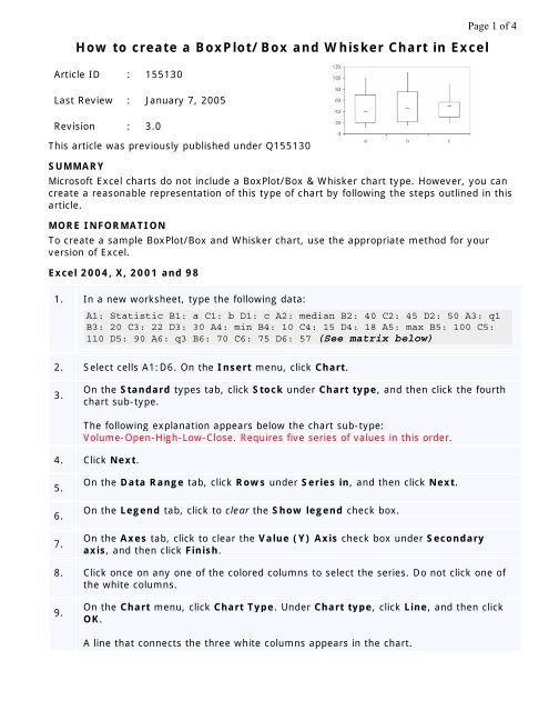
<strong>How</strong> <strong>to</strong> <strong>create</strong> a <strong><strong>Box</strong>Plot</strong>/<strong>Box</strong> <strong>and</strong> <strong>Whisker</strong> <strong>Chart</strong> <strong>in</strong> Excel<br />
Article ID : 155130<br />
Page 1 of 4<br />
Last Review : January 7, 2005<br />
Revision : 3.0<br />
This article was previously published under Q155130<br />
SUMMARY<br />
Microsoft Excel charts do not <strong>in</strong>clude a <strong><strong>Box</strong>Plot</strong>/<strong>Box</strong> & <strong>Whisker</strong> chart type. <strong>How</strong>ever, you can<br />
<strong>create</strong> a reasonable representation of this type of chart by follow<strong>in</strong>g the steps outl<strong>in</strong>ed <strong>in</strong> this<br />
article.<br />
MORE INFORMATION<br />
To <strong>create</strong> a sample <strong><strong>Box</strong>Plot</strong>/<strong>Box</strong> <strong>and</strong> <strong>Whisker</strong> chart, use the appropriate method for your<br />
version of Excel.<br />
Excel 2004, X, 2001 <strong>and</strong> 98<br />
1. In a new worksheet, type the follow<strong>in</strong>g data:<br />
A1: Statistic B1: a C1: b D1: c A2: median B2: 40 C2: 45 D2: 50 A3: q1<br />
B3: 20 C3: 22 D3: 30 A4: m<strong>in</strong> B4: 10 C4: 15 D4: 18 A5: max B5: 100 C5:<br />
110 D5: 90 A6: q3 B6: 70 C6: 75 D6: 57 (See matrix below)<br />
2. Select cells A1:D6. On the Insert menu, click <strong>Chart</strong>.<br />
3.<br />
On the St<strong>and</strong>ard types tab, click S<strong>to</strong>ck under <strong>Chart</strong> type, <strong>and</strong> then click the fourth<br />
chart sub-type.<br />
The follow<strong>in</strong>g explanation appears below the chart sub-type:<br />
Volume-Open-High-Low-Close. Requires five series of values <strong>in</strong> this order.<br />
4. Click Next.<br />
5.<br />
6.<br />
7.<br />
On the Data Range tab, click Rows under Series <strong>in</strong>, <strong>and</strong> then click Next.<br />
On the Legend tab, click <strong>to</strong> clear the Show legend check box.<br />
On the Axes tab, click <strong>to</strong> clear the Value (Y) Axis check box under Secondary<br />
axis, <strong>and</strong> then click F<strong>in</strong>ish.<br />
8. Click once on any one of the colored columns <strong>to</strong> select the series. Do not click one of<br />
the white columns.<br />
9.<br />
On the <strong>Chart</strong> menu, click <strong>Chart</strong> Type. Under <strong>Chart</strong> type, click L<strong>in</strong>e, <strong>and</strong> then click<br />
OK.<br />
A l<strong>in</strong>e that connects the three white columns appears <strong>in</strong> the chart.
Page 2 of 4<br />
10. Click once on the l<strong>in</strong>e, <strong>and</strong> then click Selected Data Series on the Format menu.<br />
For L<strong>in</strong>e select NONE; for Marker select CUSTOM, then your preference, a horizontal<br />
l<strong>in</strong>e works well; default is an “x”<br />
Step 1 Data<br />
statistic A b c<br />
median 40 45 50<br />
q1 20 22 30<br />
m<strong>in</strong> 10 15 18<br />
max 100 110 90<br />
q3 70 75 57<br />
11. You will probably want <strong>to</strong> right click <strong>in</strong> the plot area <strong>and</strong> select Format Plot Area <strong>and</strong><br />
select Area NONE. Also, get rid of the horizontal l<strong>in</strong>es by click<strong>in</strong>g near the <strong>to</strong>p <strong>and</strong><br />
under <strong>Chart</strong> Options Gridl<strong>in</strong>es, Clear Value Y Axis Major Gridl<strong>in</strong>es. (Dr. D. Recc.)<br />
120<br />
100<br />
80<br />
60<br />
40<br />
20<br />
0<br />
a b c<br />
(Acceptable, would be nice <strong>to</strong> have full l<strong>in</strong>e for the median)<br />
In Excel 2004 for Mac<br />
1. Click the Colors <strong>and</strong> L<strong>in</strong>e tab. Under L<strong>in</strong>e for Color, click No L<strong>in</strong>e.<br />
2. Under Marker, select the plus sign (+).<br />
3. In the Foreground list, click the black color. In the Background list, click No Color.<br />
Click OK.<br />
In Excel X <strong>and</strong> earlier
Page 3 of 4<br />
1. Click the Patterns tab. Under L<strong>in</strong>e, click None.<br />
2. Under Marker, click Cus<strong>to</strong>m. In the Style list, click the plus sign (+)<br />
3. In the Foreground list, click the black color.<br />
4. In the Background list, click No Color. Click OK.<br />
Excel 5.0 <strong>and</strong> Excel 7.0<br />
1. In a new worksheet, type the follow<strong>in</strong>g data:<br />
A1: Statistic B1: a C1: b D1: c A2: median B2: 40 C2: 45 D2: 50 A3: q1<br />
B3: 20 C3: 22 D3: 30 A4: m<strong>in</strong> B4: 10 C4: 15 D4: 18 A5: max B5: 100 C5:<br />
110 D5: 90 A6: q3 B6: 70 C6: 75 D6: 57<br />
2. Select cells A1:D6. On the Insert menu, po<strong>in</strong>t <strong>to</strong> <strong>Chart</strong>, <strong>and</strong> then click On This<br />
Sheet.<br />
3. Click <strong>and</strong> drag the area for the chart. In the Step 1 of 5 dialog box of the<br />
<strong>Chart</strong>Wizard, click Next.<br />
4. In the Step 2 of 5 dialog box, click the Comb<strong>in</strong>ation chart type, <strong>and</strong> then click<br />
Next.<br />
5. In the Step 3 of 5 dialog box, click the sixth chart style, <strong>and</strong> then click Next.<br />
The follow<strong>in</strong>g message appears <strong>in</strong> an Alert <strong>Box</strong>:<br />
A volume-open-high-low-close s<strong>to</strong>ck chart must conta<strong>in</strong> five series<br />
6. Click OK.<br />
7.<br />
8.<br />
In the Step 4 of 5 dialog box, click Rows under Data Series <strong>in</strong>, <strong>and</strong> then click<br />
Next.<br />
In the Step 5 of 5 dialog box, click No under Add a Legend?, <strong>and</strong> then click F<strong>in</strong>ish.<br />
9. Double-click the chart <strong>to</strong> activate it. On the Insert menu, click Axes. Under<br />
Secondary Axis, click <strong>to</strong> clear the Value (Y) Axis check box, <strong>and</strong> then click OK.<br />
10. Click once on any one of the colored columns <strong>to</strong> select the series. Do not click one of<br />
the white columns.<br />
11. On the Format menu, click <strong>Chart</strong> Type. In the list of chart types, click L<strong>in</strong>e, <strong>and</strong><br />
then click OK.<br />
A l<strong>in</strong>e that connects the three white columns appears <strong>in</strong> the chart.
Page 4 of 4<br />
12. Click once on the l<strong>in</strong>e, <strong>and</strong> then click Selected Data Series on the Format menu.<br />
13. Click the Patterns tab. Under L<strong>in</strong>e, click None.<br />
14. Under Marker, click Cus<strong>to</strong>m. In the Style list, click the plus sign (+). In the<br />
Foreground list, click the black color. In the Background list, click None. Click OK.<br />
REFERENCES<br />
Excel X <strong>and</strong> later versions:<br />
For more <strong>in</strong>formation about creat<strong>in</strong>g charts, click Excel Help on the Help menu, type about charts,<br />
click Search, <strong>and</strong> then click a <strong>to</strong>pic <strong>to</strong> view it.<br />
Excel 98 <strong>and</strong> Excel 2001<br />
For more <strong>in</strong>formation about creat<strong>in</strong>g charts, click the Office Assistant, type charts, click Search,<br />
<strong>and</strong> then click a <strong>to</strong>pic <strong>to</strong> view it.<br />
Note If the Assistant is hidden, click the Office Assistant but<strong>to</strong>n on the St<strong>and</strong>ard <strong>to</strong>olbar.<br />
Excel 7.0<br />
For more <strong>in</strong>formation about creat<strong>in</strong>g charts, click Answer Wizard on the Help menu <strong>and</strong> type:<br />
how do I <strong>create</strong> a chart<br />
Excel 5.0<br />
For more <strong>in</strong>formation about creat<strong>in</strong>g charts, choose the Search but<strong>to</strong>n <strong>in</strong> Help <strong>and</strong> type:<br />
charts<br />
APPLIES TO<br />
• Microsoft Excel 95 St<strong>and</strong>ard Edition<br />
• Microsoft Excel 5.0a<br />
• Microsoft Excel 95a<br />
• Microsoft Excel 5.0 St<strong>and</strong>ard Edition<br />
• Microsoft Excel 5.0c<br />
• Microsoft Excel 98 for Mac<strong>in</strong><strong>to</strong>sh<br />
• Microsoft Excel 5.0 for Mac<strong>in</strong><strong>to</strong>sh<br />
• Microsoft Excel 5.0a for Mac<strong>in</strong><strong>to</strong>sh<br />
• Microsoft Excel 2001 for Mac<br />
• Microsoft Excel 2004 for Mac<br />
Thanks <strong>to</strong> Laura Bruynell, <strong>Rice</strong> <strong>University</strong> STAT 280, 2/10/2005, for provid<strong>in</strong>g this reference. Source URL:<br />
http://support.microsoft.com/default.aspx?scid=kb;en-us;155130