Monge.. - SFU Wiki

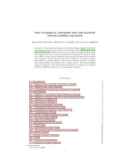
TWO NUMERICAL METHODS FOR THE ELLIPTICMONGE-AMPÈRE EQUATIONJEAN-DAVID BENAMOU, BRITTANY D. FROESE, AND ADAM M. OBERMANAbstract. The numerical solution of the elliptic Monge-Ampère Partial DifferentialEquation has been a subject of increasing interest [16, 22, 21, 9, 15, 7,8, 10, 13, 14, 12, 18]. While there are two provably convergent methods available,many of the newly proposed methods converge only for solutions whichare in H 2 (Ω), which is more regularity than is generally available for solutionsof the equation. In this article we present two methods. The first is a simplefinite difference method which is more accurate than the provably convergentwide stencil method and requires only a narrow stencil. The second methodmimics the behavior of the aforementioned methods: it performs very well forsolutions in H 2 (Ω), and poorly on more singular solutions.Contents1. Introduction 21.1. Related work: provably convergent methods 31.2. Related work: other methods 31.3. Contribution of this work, discussion of contents 42. The methods 42.1. Method 1: An Explicit Finite Difference method 42.2. Method 2: Iterative solution of the Poisson Equation 52.3. Discussion of Method 1 62.4. Discussion of Method 2 73. Numerical Examples: Overview 73.1. Comparison with previous works 73.2. Comparison of Method 1 and Method 2 83.3. Computational Details 84. Smooth or Mildly Singular Examples 94.1. An exact radial solution 94.2. Blow-up at boundary 95. Moderately Singular Examples 95.1. Noisy data 105.2. Discontinuous source term 135.3. An example which is singular at the boundary 135.4. Surface of Ball 156. Strongly Singular Examples 156.1. Cone 176.2. Absolute value function 177. Extensions to Other Methods 19Date: July 11, 2009.1

2 JEAN-DAVID BENAMOU, BRITTANY D. FROESE, AND ADAM M. OBERMAN7.1. Additional Directional Convexity 197.2. Finite Element Implementation 198. Conclusions 20References 21MA1. IntroductionThe Monge-Ampère equation is a geometric fully nonlinear elliptic Partial DifferentialEquation (PDE) [17]. Applications of the Monge-Ampère equation appear inthe classical problem of prescribed Gauss curvature and in the problem of optimalmass transportation (with quadratic cost), among others [5, 11].The numerical solution of the elliptic Monge-Ampère PDE has been a subject ofincreasing interest [22, 21, 9, 15, 7, 8, 10, 13, 14, 12, 18], including an invited lectureat 2007 ICIAM [16]. However, many of the newly proposed methods convergeonly for solutions which are in H 2 (Ω), which is more regularity than is generallyavailable for solutions of the equation. For more singular solutions, the methodsdo not converge.While one of the authors has previously introduced a convergent finite differencemethod [21], the increased attention by the numerical PDE community hasprompted us to study two methods in this paper which addresses two goals:(1) To present a simple (nine point stencil) finite difference method which performsjust as well as the provably convergent (wide stencil) method of [21]in robust numerical experiments.(2) To present a simple method which models (and outperforms) the nonconvergentmethods, and demonstrates the dramatically decreasing performanceon singular solutions.The PDE we study isdet(D 2 u(x)) = f(x),where D 2 u is the Hessian of the function u. Since we will be restricting to domainsΩ ⊂ R 2 , we can rewrite the PDE as( ∂ 2 u ∂ 2 )u(MA)∂x 2 ∂y 2 − ∂2 u(x, y) = f(x, y) in Ω ⊂ R 2 .∂x∂yThe PDE comes with Dirichlet boundary conditionsbc (D) u = g, on ∂Ωand the additional convexity constraintconvex (C) u is convexwhich is required for the equation to be elliptic. Here Ω ⊂ R n is a boundeddomain with boundary ∂Ω, and f : Ω → R is a non-negative function (or, later,measure). The PDE (MA) (along with the conditions (D, C)) is challenging tosolve numerically for the following reasons:• The equation is fully nonlinear, so weak solutions must be interpreted usingeither geometric solutions [1] or viscosity solutions [6]. In particular, theequation is not in divergence form, so there is no natural weak interpretation

TWO NUMERICAL METHODS FOR THE ELLIPTIC MONGE-AMPÈRE EQUATION 3using integration by parts. This makes the Finite Element Method (FEM)or general Galerkin projection methods unnatural for the problem.• The weak solutions of the equation can be quite singular. Specifically, theyare not in H 2 (Ω). In fact, they may be only Lipschitz continuous 6.1.• The convexity constraint: the solution u must be convex in order for theequation to be elliptic. Without the convexity constraint, this equation doesnot have a unique solution. (For example, taking boundary data g = 0, ifu is a solution then −u is also a solution, in R 2 .)1.1. Related work: provably convergent methods. Two provably convergentmethods have already been presented for (MA).The first, by Oliker and Prussner [22], uses a discretisation based on the geometricinterpretation of the solutions [1]. In two dimensions this method converges tothe geometric solution.The second, by one of authors of this work [21], converges to the viscosity solutionof (MA). While it is not difficult to build consistent, stable numerical methodsfor (MA), this alone is not enough to prove convergence to the viscosity solution. Forconvergence of approximation methods to the viscosity solution, another ingredientis needed, namely monotonicity of the methods [2]. Monotone methods respectthe comparison principle at the discrete level [19]. However, building monotonemethods for this equation requires the use of wide stencils, which come with anadditional consistency error related to the directional resolution of the stencil.1.2. Related work: other methods. There have been a number of other recentlyproposed methods. We emphasise the point that consistency and stability alone arenot enough to ensure convergence to either the geometric or viscosity solution. Inparticular, as explained by Dean and Glowinksi (see below), in the case wheresolutions are not in H 2 (Ω), finite element or Galerkin methods do not converge.Dean and Glowinski et al. [9, 15, 7, 8, 10, 16] have investigated Lagrangian andleast squares methods for the numerical solution of Monge-Ampère. The authorsare careful to be clear about the convergence behavior of their methods. In [8] theygive an example of a solution that is not in H 2 (Ω) for which their method diverges.They point out in [7] “if, despite the smoothness of its data, the above problemhas no solution in H 2 (Ω), the above augmented Lagrangian method solves it in aleast-squares sense,” and in [8], “in cases where the Monge-Ampère equation underconsideration has no smooth solution, [the methods] provide a quasi-solution”.Feng and Neilan [13, 14], solve second order equations (including the Monge-Ampère equation) by adding a small multiple of the bilaplacian. Although notstated explicitly, their method appears to require that solutions be in H 2 (Ω). Thehigher order terms require boundary conditions, and it is not explained how theseadditional boundary conditions are compatible with the solution. They have citeda proof of convergence, but at the time of revision of this work it was not yetavailable.Loeper and Rapetti [18] solve the equation (with periodic boundary conditions)by linearisation and iterate using Newton’s method. They prove convergence of theNewton algorithm for the linearisation of the continuous problem to the solutionof (MA). However, they do not address the issue of the convergence of the discretisedsolution to the solution of the equation in the limit of the discretisationparameter going to zero.

4 JEAN-DAVID BENAMOU, BRITTANY D. FROESE, AND ADAM M. OBERMANBöhmer [3] performs consistency and stability analysis of finite element methodsfor fully nonlinear equations.1.3. Contribution of this work, discussion of contents. Motivated by theinterest in the problem, we propose in §2 two different numerical methods for solving(MA). These methods have the advantages of simplicity and performance.The methods are simple in the sense that the algorithms are fully explained inabout a page, and can be implemented in MATLAB using only basic explicit matrixoperations (M1,M2) and a linear solve (M2).First, we set out to build the simplest possible finite difference method for (MA).Our original goal was to find an example where the monotone method of [21] converged,and the finite difference method (M1) diverged. In fact, we found that themethod (M1) converged for all the examples we tried. In addition, this method issecond order accurate (whch is better than the wide stencil method) and is simplyimplemented on a nine point stencil. However, the method is not monotone, so noconvergence proof is available for the method. Based on the success of this method,we take the point of view that the convergent method [21] can be used to validatethe more efficient non-provably convergent method (M1).Second, while we did not undertake to directly implement the methods by Deanand Glowinksi, or Feng and Neilan, we devised a method which can be interpretedas a model for their schemes in the sense that it requires solutions to be in H 2 (Ω).The resulting method is (M2).This performance of (M2) relative to (M1) is superior when the solutions aresmooth but substantially inferior when the solutions are singular. In fact, we havefound strongly singular solutions for which (M2) appears to diverge.The overall and relative performance of the methods is summarised and discussedin §3. We study in detail the performance of the two methods on solutions rangingfrom smooth §4 to moderate §5 to very singular §6.The only case where the monotone method was superior to (M1) was for themost singular example computed, §6.1. In this case, the first method, (M1), was lessaccurate than the monotone method. A minor modification (implemented in §7.1)improves the accuracy of the method by an order of magnitude while maintaininga narrow stencil. Other extensions are discussed in §7.sec:Methods2. The methodsIn this section we present the two methods for solving the two-dimensionalMonge-Ampère equation. The first is an explicit, Gauss-Seidel iteration methodthat is obtained by solving a quadratic equation at each grid point and choosingthe smaller root to ensure selection of the convex solution.The second method is an iterative method which requires the solution of a Poissonequation at each iteration. The source term in the Poisson equation involvesthe source function for (MA), f, and the Hessian of the current iterate.2.1. Method 1: An Explicit Finite Difference method. The first methodinvolves simply discretising the second derivatives in (MA) using standard centraldifferences on a uniform Cartesian grid. The result isMAdiscrete (2.1) (Dxxu 2 ij )(Dyyu 2 ij ) − (Dxyu 2 ij ) 2 = f i,j

TWO NUMERICAL METHODS FOR THE ELLIPTIC MONGE-AMPÈRE EQUATION 5wheredef_d (2.2)D 2 xxu ij = 1 h 2 (u i+1,j + u i−1,j − 2u i,j )D 2 yyu ij = 1 h 2 (u i,j+1 + u i,j−1 − 2u i,j )D 2 xyu ij = 14h 2 (u i+1,j+1 + u i−1,j−1 − u i−1,j+1 − u i+1,j−1 )Since we are using centred differences, this discretisation is consistent with (MA),and it is second order accurate.Next, introduce the notationa 1 = (u i+1,j + u i−1,j )/2a 2 = (u i,j+1 + u i,j−1 )/2a 3 = (u i+1,j+1 + u i−1,j−1 )/2a 4 = (u i−1,j+1 + u i+1,j−1 )/2and rewrite (2.1) as a quadratic equation for u i,j4(a 1 − u i,j )(a 2 − u i,j ) − 1 4 (a 3 − a 4 ) 2 = h 4 f i,j .Solving for u i,j and selecting the smaller root (in order to select the locally convexsolution), we obtain Method 1:√M1 (M1) u i,j = 1 2 (a 1 + a 2 ) − 1 2(a 1 − a 2 ) 2 + 1 4 (a 3 − a 4 ) 2 + h 4 f i,jWe can now use Gauss-Seidel iteration to find the fixed point of (M1). TheDirichlet boundary conditions (D) are enforced at boundary grid points. Theconvexity constraint (C) is not enforced beyond the selection of the positive rootin (M1)def:Op2.2. Method 2: Iterative solution of the Poisson Equation. The secondmethod we study involves successively solving the Poisson equation until a fixedpoint is reached. This method is a model for the non-convergent methods whichrequire that the solution be in H 2 (Ω).The method is based on an algebraic identity satisfied by the two-dimensionalMonge-Ampère equation, used by Dean and Glowinski [9, 15, 7, 8, 10]. We generalisethis idea below to produce a fixed point operator in higher dimensions.Expanding (∆u) 2 = (u xx + u yy ) 2 and applying (MA), we obtain the identity(u xx + u yy ) 2 = u 2 xx + u 2 yy + 2u 2 xy + 2ffor solutions u(x, y) of (MA) which are smooth enough.This algebraic identity leads to the following definition, where the positive squareroot is selected in order to select the locally convex solution.Definition 1. Define the operator T : H 2 (Ω) → H 2 (Ω) for Ω ⊂ R n( by√ )T [u] = ∆ −1 (∆u)2 + 2(f − det(D 2 u)) .In particular, in R 2 ,(√ )eq:Op2d (2.3) T [u] = ∆ −1 u 2 xx + u 2 yy + 2u 2 xy + 2f .

6 JEAN-DAVID BENAMOU, BRITTANY D. FROESE, AND ADAM M. OBERMANlem:Op2dThe solution operator incorporates the Dirichlet boundary conditions (D).Remark. While it is possible to define the domain of the operator more carefully,for our purposes it is sufficient to observe the it is well-posed on H 2 (Ω).Lemma 1. Provided the solution, u, of (MA) is in H 2 (Ω), it is a fixed point of theoperator T .Proof. Let v be the solution of (MA, D, C). Since v is in H 2 (Ω), ∆v is in L 2 (Ω)and the Poisson equation∆u = |∆v| ,augmented by the Dirichlet boundary conditions (D), is well-posed. Inserting thesolution v into Definition 1 we obtain( √ )T [v] = ∆ −1 (∆v)2= ∆ −1 (|∆v|).Since v is convex, by (C), ∆v > 0, and consequently,Therefore, v is a fixed point of (M2).T [v] = ∆ −1 (∆v) = v.Method 2 consists of iterating u n+1 = T [u n ] by solving√M2 (M2) ∆u n+1 = (u n xx) 2 + (u n yy) 2 + 2(u n xy) 2 + 2f.along with the prescribed Dirichlet boundary conditions (D).2.3. Discussion of Method 1. In order to prove convergence of the finite differentmethod to viscosity solution of (MA), it is sufficient to prove that the method ismonotone. When written in the form (M1), it would be enough to show [19] thatthe value u i,j is a non-decreasing function of the neighboring values. However, thisis not the case for (M1). In addition, based on the discussion in [21] and [20] wedon’t expect that any narrow stencil method will be monotone and consistent forthe equation (MA).However, we can study the convexity requirement. Directional convexity alonggrid directions is the requirement that the solution satisfyu(x + v) + u(x − v)eq:convex (2.4) u(x) ≤2for all lattice (grid) directions v. For more details about enforcing convexity ofsolutions, using finite difference methods, we refer to [20].The directional convexity along the axes is satisfied by (M1).lem:conv1Lemma 2. The fixed point of (M1) satisfies the inequalities (2.4) for the grid directionsv ∈ {(1, 0), (0, 1)}.Proof. Using the notation of (2.2), assume without loss of generality that a 2 ≤ a 1 .Next, estimate u i,j from (M1), using the fact that f is non-negative,u i,j ≤ a 1 + a 2− a 1 − a 2= a 2 = u i,j+1 + u i,j−12 22to obtain convexity in the direction v = (1, 0). Using the first assumption in theproof, we also haveu i,j ≤ u i+1,j + u i−1,j,2□

TWO NUMERICAL METHODS FOR THE ELLIPTIC MONGE-AMPÈRE EQUATION 7which gives the convexity in the direction v = (0, 1).2.4. Discussion of Method 2. The method is convenient to implement because itsimply involves evaluating derivatives, and solving the Poisson equation, which canbe performed using the method of choice. However, the Poisson equation is solvedwith a source involving the norm of the Hessian of the previous solution. Whenthe solution is not in H 2 (Ω), this function can be unbounded. The regularityrequirement for solutions makes the the method is a model for the Finite Elementand Galerkin methods discussed in the introduction, because they require solutionsto be in H 2 (Ω) for convergence.□sec:overview3. Numerical Examples: OverviewIn this section we discuss the performance of the methods on a range of computationalexamples. These examples fall into three categories depending on theregularity of the solution.• Smooth or mildly singular solutions. These solutions are the mildest: weexpect any reasonable methods for Monge-Ampère will perform well. Inthese cases we find that (M2) is faster than (M1) by more than an order ofmagnitude.• Moderately singular solutions. These examples that are at the edge of thecapabilities of many of the existing methods. Both of our methods producesimilar results.• Strongly singular solutions. In this case many of the methods currentlyavailable either have not demonstrated convergence, or, as in the case of [9,15, 7, 8, 10], are known to fail. For these examples, at a given, finite,resolution, (M1) converges more quickly than (M2) by a couple of orders ofmagnitude. The effect is more substantial at the higher resolutions tested.The increasingly slow convergence rate for (M2) (both compared to (M1)and to (M2) on smoother solutions) is consistent with divergence.Regularity results can be used to determine when solutions are in H 2 (Ω), andthereby determine the method of choice. For strictly convex domains and smoothstrictly positive data, the solution is smooth [4]. However, as soon at f approacheszero, regularity breaks down, see [17] for W 2,p estimates on solutions.3.1. Comparison with previous works. There are four main examples computedby Dean and Glowinski. Feng and Neilan give computational examples forthe first three problems, but not the fourth. The first two, which are we callmild, are studied in §4.1,4.2. The third, for which no exact solution is available,but the solution is known to be singular, is studied in 5.3. The fourth solution isnot in H 2 (Ω). For this solution, the method of Dean and Glowinski diverges [8,p.1361], and Feng and Neilan did not present computational examples. While theconvegence rate is slower than for the smoother examples, both our methods (M1)and (M2) appear to converge for this example, §5.4.The solutions above we categorize as mild or moderate. In addition, we alsopresent computational results for more singular examples, §6.We compare the results of Dean and Glowinksi [9, 15, 7, 8, 10] to (M2), whichis the model for these methods. For the first three examples, these require roughlythe same number of iterations to converge. Although computation times were notgiven, presumably, each iteration of our method is more efficient, since it involves a

8 JEAN-DAVID BENAMOU, BRITTANY D. FROESE, AND ADAM M. OBERMANsingle Poisson solve. Each iteration of [9, 15, 7, 8, 10] involves a Poisson solve andadditional calculations.Feng and Neilan [14, 12, 13] do not give details about the computation time oriteration count of their numerical method.3.2. Comparison of Method 1 and Method 2. The computation time for (M1)was roughly independent of the regularity of the solution. On the other hand, thecomputation times for (M2) were faster (by more than one order of magnitude) onvery smooth solutions, about equal on mildly singular solutions, and much slower(by a couple of orders of magnitude) on the more singular solutions.Naturally, for any finite resolution, the discretised solutions are not singular, sowe cannot conclude that the method diverges. But since the relative computationalcosts increase dramatically as the solutions become less regular, this behavior isconsistent with divergence.We find (M2) performs extremely rapidly when solutions are smooth, but isvery slow when solutions are not smooth or not strictly convex. The explicitmethod (M1), on the other hand, requires approximately the same amount of CPUtime to converge without regard for the regularity of the solutions.To show this more concretely, we consider a representative example from eachcategory: the smooth radial solution of §4.1, the example with noisy data of §5.1,and the non-smooth cone of §6.1. We compare the absolute computation timerequired for these three examples to demonstrate our observation that the speedof (M1) is independent of regularity while the speed of (M2) is very sensitive toregularity; see Figure 1. We compare the ratio of CPU times required by the twomethods for a representative example, see Table 1.(a)fig:Meth1(b)fig:Meth2Figure 1. CPU time required to converge for the smooth radialsolution of §4.1, the noisy solution of §5.1, and the non-smoothcone of §6.1. (a) Results for (M1). (b) Results for (M2).fig:times3.3. Computational Details. The solutions are computed on an N × N gridand iteration is continued until the maximum difference between two subsequentiterates is less than 10 −14 . By convention, h is the spatial discretisation parameterh = L/N where L is the length of one side of the square domain.

TWO NUMERICAL METHODS FOR THE ELLIPTIC MONGE-AMPÈRE EQUATION 9table:ratiosN §4.1 §5.1 §6.121 6.3 1.3 .1241 4.1 2.1 .0761 7.7 1.9 .0681 11.7 1.5 .05101 14.1 1.2 .04121 23.5 1.0 .07141 29.9 .7 .05Table 1. Ratio of computation times required for (M1) and (M2)for three representative examples: the smooth radial solution of§4.1, the noisy solution of §5.1, and the non-smooth cone of §6.1.A reasonable choice for the initial data is the solution of u xx + u yy = √ 2f,which was used when measuring the solution time and iteration count. However,the methods are robust: the iterations converge to a fixed point for all initial dataattempted. The initial data attempted included: a constant (which didn’t respectthe boundary conditions), and both non-convex and random initial data.The implementation of (M2) can be performed using the method of choice. Wefocus on the simple finite difference method which arises from discretising (2.3)using central differences (as with the first method). We also briefly discuss in §7.2the use of an adaptive finite element method.sec:smoothsec:radialsec:blowupsec:moderate4. Smooth or Mildly Singular ExamplesIn the following examples, the solutions are smooth, or mildly singular, and (M2)is much faster than (M1). We observed convergence rates consistent with of O(h 2 )for the smooth solution, and O(h 1.5 ) for the mildly singular solution.4.1. An exact radial solution. An exact radial solution is( x 2 + y 2 )u(x, y) = exp, f(x, y) = (1 + x 2 + y 2 ) exp(x 2 + y 2 ).2Both methods converge to the same numerical solution, which is accurate to secondorder in h, O(h 2 ), see Figure 2(a). For this smooth example, (M2) is by far thefastest method: see Table 2 and Figure 2(b).4.2. Blow-up at boundary. Another exact solution isu(x, y) = 2√ 23 (x2 + y 2 ) 3/4 1, f(x, y) = √x2 + y 2on the square [0, 1] × [0, 1]; the function f blows up at the boundary. Again, bothmethods converge to the exact solution, although the order of convergence is nowonly 1.5. For this example (M2) was significantly faster than (M1). See Tables 3and 4 and Figure 3.5. Moderately Singular ExamplesIn the following examples, the solutions are moderately singular, and the twomethods perform about equally.

10 JEAN-DAVID BENAMOU, BRITTANY D. FROESE, AND ADAM M. OBERMAN(a)fig:errinf1(b)fig:time1Figure 2. Convergence results for u(x, y) = exp(x 2 +y 2N × N grid. (a) Error versus N. (b) Total CPU time.2)on anfig:ex1table:ex1_2N Iterations CPU Time (sec)(M1) (M2) (M1) (M2)21 1014 54 .9 0.181 14621 59 39.8 3.4141 42746 60 350.0 11.7201 84611 60 1540.0 27.2261 — 65 — 57.8......341 — 65 — 118.0421 — 78 — 249.0501 — 151 — 804.0581 — 284 — 2120.0Table ( 2. ) Computation times for the exact solution u(x, y) =exp x 2 +y 2on an N × N grid.2N 21 61 101 141 181 221∥∥u − u (N)∥ ∥∞5.5 × 10 −4 1.1 × 10 −4 5.0 × 10 −5 3.0 × 10 −5 2.1 × 10 −5 1.5 × 10 −5table:ex9Table 3. Errors for the exact solution u(x, y) = 2√ 23 (x2 + y 2 ) 3/4on an N × N grid. Results are the same for both methods.sec:noisy5.1. Noisy data. We now return to the first example we considered, with exactsolution( x 2 + y 2 )u(x, y) = exp, f(x, y) = (1 + x 2 + y 2 ) exp(x 2 + y 2 ),2

TWO NUMERICAL METHODS FOR THE ELLIPTIC MONGE-AMPÈRE EQUATION 11(a)fig:f9(b)fig:sol9(c)fig:err9(d)fig:time9Figure 3. Results for u(x, y) = 2√ 23 (x2 +y 2 ) 3/4 on an N ×N grid.(a) f blows up at the boundary. (b) Surface plot of the solution.(c) Error versus N. (d) Total CPU time.fig:ex9table:ex9_2N Iterations CPU Time (sec)(M1) (M2) (M1) (M2)21 1083 58 .5 .261 8967 59 28.7 1.9101 23849 59 206.0 6.9141 45358 59 770.0 11.4181 73254 59 2050.0 21.2221 107388 60 4500.0 34.6Table 4. Computation times for u(x, y) = 2√ 23 (x2 + y 2 ) 3/4 on anN × N grid.and study the effects of adding high frequency sinusoidal noise to the data (f andthe boundary conditions). Results are shown in Figure 4. Although the data isnot convex, all methods find a solution that is convex except at the boundary.The noise does not seem to have any effect on the rate of convergence for (M1).However, (M2) becomes much slower when dealing with the noisy, non-convex data

12 JEAN-DAVID BENAMOU, BRITTANY D. FROESE, AND ADAM M. OBERMANso that the time required for the two methods is comparable; compare Tables 2and 5.(a)fig:f1(b)fig:f14(c)fig:sol14(d)fig:err14Figure 4. Results for u(x, y) = exp(x 2 +y 22)with noisy, nonconvexdata on an 81 × 81 grid. (a) f without noise. (b) f with∣ ∣ ∣∣noise. (c) Surface plot of the solution with noise. (d) ∣u − u noisyfig:ex14table:ex14N Iterations CPU Time (sec)(M1) (M2) (M1) (M2)21 1016 58 .2 0.141 3866 99 2.4 1.261 8432 185 10.7 5.681 14672 409 32.0 21.0101 22516 695 77.6 63.4121 31965 1205 153.0 156.0141 43008 2162 291.0 401.0Table 5. Computation times for u(x, y) = expnoisy data on an N × N grid.(x 2 +y 22)with

TWO NUMERICAL METHODS FOR THE ELLIPTIC MONGE-AMPÈRE EQUATION 13sec:discts5.2. Discontinuous source term. We next consider an example source term fthat is discontinuous on a circle{1 (x − 0.5) 2 + (y − 0.5) 2 > 0.16 2f =0 otherwise.The solution is{ (x − 0.5) 2 + (y − 0.5) 2 }u = max, 0.08 .2The solution is flat where f vanishes and parabolic elsewhere. See the surface plotin Figure 5(a). Both methods require about the same amount of time for thisexample as is seen in Figure 5(b) and Table 6.fig:ex15(a)fig:sol15(b)fig:time15Figure 5. Results for §5.2. (a)Surface plot of solution. (b) TotalCPU time.table:ex15N Iterations CPU Time (sec)(M1) (M2) (M1) (M2)21 950 90 0.2 0.341 3651 259 2.0 3.461 7944 363 9.4 12.181 13810 783 21.5 42.5101 21162 893 68.0 85.0121 29966 1678 132.0 221.0141 40196 2076 244.0 480.0Table 6. Computation times for §5.2 on an N × N grid.sec:nonsmooth5.3. An example which is singular at the boundary. This example was takenfrom [8] We consider the solution of Monge-Ampère when f = 1 with constantboundary values 1 on the square [−1, 1]×[−1, 1]. There is no exact solution availablefor this example, however the solution is not smooth: since u xx = 0 on part of theboundary, u yy → ∞ there. Method (M1) converges to a solution that is convexexcept near the corners of the domain (Figure 6(b)). This is comparable to the

14 JEAN-DAVID BENAMOU, BRITTANY D. FROESE, AND ADAM M. OBERMANsolutions presented in [8]. Method (M2) converges to a slightly different, moreconvex, solution.As no exact solution is available for comparison, following [21], we focus on theminimum value of the solution produced by each method. We also consider theminimum values obtained using the monotone method in [21]; see Table 7. Thesolutions obtained with our methods are lower than the solutions obtained with themonotone, wide-stencil method. The monotone method is known to converge toa supersolution of (MA), so we do expect these values to be higher than the truevalues. This is evident in the numerics as the solution obtained with the monotonemethod becomes lower (and closer to the solutions obtained with our methods) asthe stencil width is increased.Method (M2) performs very slowly in this case. It is also much slower than (M1),which requires about the same number of iterations to converge as it did for thesmooth examples. See Figure 7 and Table 8.(a)fig:sol2(b)fig:corner2Figure 6. Solutions when f = 1 with constant boundary values 1.(a) Surface plot of solution. (b) The methods produces a solutionwith slight negative curvature along the line y = x.fig:ex2table:ex2Nu (N)min(M1), 9-Point 17-Point 33-Point(M2) Stencil Stencil Stencil21 0.2892 0.3115 0.2815 0.283941 0.2734 0.3090 0.2807 0.273261 0.2682 0.3082 0.2803 0.271181 0.2655 0.3078 0.2802 0.2704101 0.2639 0.3076 0.2800 0.2700121 0.2629 0.3075 0.2798 0.2697141 0.2621 0.3074 0.2796 0.2695Table 7. Minimum value of u when f = 1 with constant boundaryvalues 1 on an N ×N grid. We include results from the wide stencilmethods of [21] on nine, seventeen, and thirty-three point stencils.

TWO NUMERICAL METHODS FOR THE ELLIPTIC MONGE-AMPÈRE EQUATION 15(a)fig:its2(b)fig:time2Figure 7. Convergence results when f = 1 with constant boundaryvalues 1 on an N × N grid. (a) Total number of iterationsrequired verus N. (b) Total CPU time versus N.fig:ex2_2table:ex2_2N Iterations CPU Time (sec)(M1) (M2) (M1) (M2)21 1615 535 .1 1.741 6366 1917 .6 33.661 14049 4070 2.8 254.081 24560 6944 8.1 1170.0101 37824 10503 19.9 3730.0121 53778 14711 41.2 6820.0141 72377 19571 99.7 8560.0Table 8. Computation times when f = 1 with constant boundaryvalues 1 on an N × N grid.sec:ballsec:singular5.4. Surface of Ball. Next we consider another example from [8], which is theexact solutionu(x, y) = − √ 2 − x 2 − y 2 2, f =(2 − x 2 − y 2 ) 2on the domain [0, 1] × [0, 1]. The method of [8] is known to diverge for this example,however both (M1) and (M2) successfully capture this non-smooth solution,although we no longer have second order accuracy as we did with the smooth solutionof §4.1, instead the convergence rate is about .5. See Figure 8 and Table 9. Inthis case (M2) outperforms (M1) by an order of magnitude with regard to computationtime.6. Strongly Singular ExamplesIn the following examples, the solutions are strongly singular (they are not inH 2 (Ω)), and (M2) is expected to diverge. The increasingly large number of iterationsrequired to locate a fixed point of (M2) (both relative to (M1) on the samesolutions, and relative to (M2) on smoother solutions) is consistent with divergence.

16 JEAN-DAVID BENAMOU, BRITTANY D. FROESE, AND ADAM M. OBERMAN(a)fig:sol_ball(b)fig:err_ball(c)fig:its_ball(d)fig:time_ballFigure 8. Results for u(x, y) = − √ 2 − x 2 − y 2 on an N ×N grid.(a) Surface plot of the solution. (b) Error versus N. (c) Numberof iterations. (d) Total CPU time.fig:balltable:ballN Iterations CPU Time (sec)(M1) (M2) (M1) (M2)21 1009 67 .2 .241 3833 79 1.9 1.061 8343 89 8.5 2.781 14480 99 26.3 5.2101 22189 106 60.2 10.0121 31445 113 120.1 15.0141 42202 119 218.3 21.3Table 9. Computation times when u = − √ 2 − x 2 − y 2 on anN × N grid.For the cone u(x, y) = √ x 2 + y 2 , the convergence rate decreases to O(h .8 ), andthe solution time is about one order of magnitude slower for (M2).Another example is the absolute value function u(x, y) = |x| in §6.2. Here thecomputation time for (M1) is two orders of magnitude faster than for (M2). Sincethe solution is piecewise linear, the discretisation error is zero. However, the rate

TWO NUMERICAL METHODS FOR THE ELLIPTIC MONGE-AMPÈRE EQUATION 17sec:coneof convergence for iterations to a fixed point is O(N −5 ) for (M1) and the O(N −2 )for (M2).6.1. Cone. Next we consider the cone u(x, y) = √ x 2 + y 2 . To obtain this solutionwith our methods we set f to be the appropriately weighted delta distribution atthe origin, which discretises to{4/h 2 x i = y j = 0f i,j =0 otherwise,(centering the grid so that the origin is a grid point), so that (MA) is satisfiedin the sense of distributions. Despite the fact that this solution is only Lipschitzcontinuous, both still converge to the exact solution; see Table 10 and Figure 9,however the rate of convergence is approximately O(h .8 ) and the computationaltime for (M2) is about two orders of magnitude longer than for (M1) (Table 11).(a)fig:sol10(b)fig:err10(c)fig:its10(d)fig:time10Figure 9. Results for u(x, y) = √ x 2 + y 2 on an N × N grid. (a)Surface plot of the solution. (b) Error versus N. (c) Total numberof iterations. (d) Total CPU time.fig:ex10sec:abs6.2. Absolute value function. Next we consider the function u(x, y) = |x|, whichis Lipschitz continuous but not differentiable. Since even at the edge one eigenvalueis zero, det(D 2 u) = 0 in the sense of distributions. Therefore setting f = 0,

18 JEAN-DAVID BENAMOU, BRITTANY D. FROESE, AND ADAM M. OBERMANN 21 61 101 141∥ u − u(N) ∥ ∥∞1.4 × 10 −2 5.9 × 10 −3 3.8 × 10 −3 2.8 × 10 −3table:ex10Table 10. Errors for the exact solution u(x, y) = √ x 2 + y 2 on anN × N grid.table:ex10_2N Iterations CPU Time (sec)(M1) (M2) (M1) (M2)21 1148 424 0.1 1.141 4386 1458 2.5 35.661 9588 3017 11.4 200.081 16686 5082 33.2 681.0101 25635 7561 73.3 2090.0121 36396 10486 235.0 3560.0141 48946 13750 372.0 7160.0Table 11. Computation times for u(x, y) = √ x 2 + y 2 on an N ×N grid.all methods correctly find this solution. Moreover, it appears that regardless ofthe value of N, the error in the approximations can be made arbitrarily small byiterating sufficiently many times (since the solution is piecewise linear).Although all three methods appear to be exact for this example, (M1) performsmuch more quickly for this degenerate example. We plot maximum error againstnumber of iterations in Figure 10(b). From this plot we observe that the errordecreases like the fifth power of the number of iterations for (M1), but only decreasesquadratically for (M2). The difference in computational time is even morepronounced; see Table 12.fig:sol4Figure 10. Results for u(x) = |x| on an N × N grid. (a) SurfacePlot. (b) Error versus number of iterations for N = 81.fig:err4fig:ex4

TWO NUMERICAL METHODS FOR THE ELLIPTIC MONGE-AMPÈRE EQUATION 19table:ex4N Iterations CPU Time (sec)(M1) (M2) (M1) (M2)21 1417 3604 .2 941 5366 13252 1.9 16461 11636 28233 12.0 87881 20135 48116 37.3 2440101 30795 72727 83.2 6650Table 12. Computation times for u(x, y) = |x| on an N × N grid.sec:extensionssec:M1b7. Extensions to Other MethodsSeveral modifications to our methods can be used to improve the results in someof the non-smooth examples.7.1. Additional Directional Convexity. The convergent finite difference methodof [21] enforced directional convexity in many directions by using a wide stencilmethod. The purpose of this section is the explore whether increasing the directionsof convexity, while maintaining a narrow stencil improves the methods.Along the lines of [21] and [20] (where convexity along several directions ensuresconvergence), we can also build more convexity requirements into our method. Thisis accomplished by modifying (M1) as follows.Method1b (M1 ∗ ) ⎧ √ ⎫⎨(a1 ) 2 ( ) 2a 1 + a 2 − a 2 a3 − a 4u i,j = min −++ 1 ⎬⎩ 224 4 f i,jh 4 , a 3 , a 4⎭ .lem:conv2sec:FEMLemma 3. The fixed point of (M1 ∗ ) satisfies the inequality (2.4) for the grid directionsv ∈ {(1, 0), (0, 1), (−1, 1), (1, 1)}.Proof. The proof of the first part of this lemma is the same as the proof of the firstpart of Lemma 2. The second half of this lemma is built directly into (M1 ∗ ). □In the majority of cases, this modified method performs comparably (or identically)to (M1), with both methods converging to the same solution. One notableexception to this trend is the cone. Although the convergence time is the same forboth (M1) and (M1 ∗ ), the results obtained with (M1 ∗ ) are roughly one order ofmagnitude more accurate; see Table 13.7.2. Finite Element Implementation. The Method (M2) involves iterativelysolving Poisson’s equation. The Poisson solver can be implemented using themethod of choice. We tried a finite element solver which took advantage of meshadaptation, to see if the performance of the method improved.We implemented the Poisson sovler of (M2) using a Finite Element LagrangianP 2 Poisson solver, FreeFem++. This software incorporates an anisotropic meshadaptative algorithm. At each iteration of (M2) we the mesh is adapted based onbased on the magnitude of the norm of the Hessian of the solution. All computationsstart on a uniform mesh with a total of M elements. Mesh adaptation changes thenumber of elements. However, we can roughly control the number of elements usingthe parameter h min (which specifies the minimum size of an element).

IsoValue-0.18101-0.171727-0.162445-0.153162-0.14388-0.134597-0.125315-0.116032-0.106749-0.0974669-0.0881843-0.0789018-0.0696192-0.0603366-0.0510541-0.0417715-0.032489-0.0232064-0.0139238-0.00464128table:cone20 JEAN-DAVID BENAMOU, BRITTANY D. FROESE, AND ADAM M. OBERMANN∥ ∥ u − u(N) ∞(M1) (M1 ∗ )21 1.4 × 10 −2 2.5 × 10 −341 8.2 × 10 −3 1.5 × 10 −361 5.9 × 10 −3 1.1 × 10 −381 4.6 × 10 −3 8.4 × 10 −4101 3.8 × 10 −3 7.0 × 10 −4121 3.2 × 10 −3 6.0 × 10 −4141 2.8 × 10 −3 5.3 × 10 −4Table 13. Errors for the exact solution u(x, y) = √ x 2 + y 2 on anN × N grid.We monitor the difference between two succesive iterates, called convergencebelow, to check that the iterative process converges. Finally, we monitor the residualdefined as√R[u] = ∆T [u] − u 2 xx + u 2 yy + 2u 2 xy + 2f,which should go to 0 as we reach the solution of Monge-Ampère.In most examples, this finite element implementation is not significantly fasterthan the finite difference implementation. The adaptivity improved performance forthe example of §5.3. This method, initialised on a uniform 40×40 mesh, converges inabout 40 iterations whereas the finite difference implementation requires thousandsof iterations to converge. See Figure 11 and Table 8.(a)fig:nonsmooth_sol(b)fig:nonsmooth_convFigure 11. Results with f = 1 and homogeneous Dirichlet boundaryconditions initialised on a uniform 40 × 40 mesh. (a) Finalmesh and level curves of the solution. (b) Convergence and residualagainst number of iterations.fig:nonsmooth8. ConclusionsTwo simple numerical methods (M1), (M2) were introduced for solving (MA).Computations were performed on a number of solutions whose regularity ranged

TWO NUMERICAL METHODS FOR THE ELLIPTIC MONGE-AMPÈRE EQUATION 21from smooth to strongly singular. Iteration counts and computation times weremeasured for both methods. Performance comparisons were made between the twomethods, and, as much as possible, between results available for existing methods.The first, (M1), is a simple explicit finite difference method. While it is secondorder accurate, it is not monotone, so there is no convergence proof available. However,the method appeared to converge for all the numerical examples computed.These examples ranged from very smooth to singular (not in H 2 (Ω), Lipschitzcontinuous). The discrete equation was solved by a simple iterative method, andthe number of iterations (for fixed problem size) was roughly independent of theregularity of solution.We concluded that method, which is simply the natural finite difference discretizationof the equation, is the simplest and best performing method currentlyavailable, for generic problems. Only in the most singular case studied did theprovably convergent method of [21] perform better. However, in this case, we introduceda simple modification of (M1) which improved accuracy by an order ofmagnitude, §7.1.The second method used an algebraic identity satisfied by (MA) to write the solutionof the equation in terms of the Laplacian of a function of the norm of the Hessianof the solution and the source term (2.3). This led to an iterative method (M2)which required successive solutions of a Poisson equation. This method is simple toimplement and demonstrably superior to the other methods which required solutionsto be in H 2 (Ω). While the method of Dean and Glowinksi failed to convergefor a particular solution not in H 2 (Ω), (M2) converged for this example (althoughthe accuracy was less than for the smoother examples). Comparing the convergentexamples, the number of iterations to converge was about the same for both methods,but each iteration of (M2) is simpler because it involves only the solution of aPoisson equation.Compared to Method (M1), Method (M2) was faster (by at least an order ofmagnitude) on smooth solutions. However, strongly singular solutions led to apoorly conditioned Poisson equation, and (M2) it was slower (by more than anorder of magnitude) than (M1) on the most singular solutions.So we conclude that Method (M2) is the method of choice for solutions whichare known to be in H 2 (Ω) or better, while Method (M1) is the method of choicefor generic problems.References[1] I. Bakelman. Convex analysis and nonlinear geometric elliptic equations. Springer-Verlag,1994.[2] Guy Barles and Panagiotis E. Souganidis. Convergence of approximation schemes for fullynonlinear second order equations. Asymptotic Anal., 4(3):271–283, 1991.[3] Klaus Böhmer. On finite element methods for fully nonlinear elliptic equations of secondorder. SIAM J. Numer. Anal., 46(3):1212–1249, 2008.[4] L. Caffarelli, L. Nirenberg, and J. Spruck. The Dirichlet problem for nonlinear second-orderelliptic equations. I. Monge-Ampère equation. Comm. Pure Appl. Math., 37(3):369–402, 1984.[5] Luis A. Caffarelli and Mario Milman, editors. Monge Ampère equation: applications to geometryand optimization, volume 226 of Contemporary Mathematics, Providence, RI, 1999.American Mathematical Society.[6] Michael G. Crandall, Hitoshi Ishii, and Pierre-Louis Lions. User’s guide to viscosity solutionsof second order partial differential equations. Bull. Amer. Math. Soc. (N.S.), 27(1):1–67,1992.

22 JEAN-DAVID BENAMOU, BRITTANY D. FROESE, AND ADAM M. OBERMAN[7] E. J. Dean and R. Glowinski. An augmented Lagrangian approach to the numerical solutionof the Dirichlet problem for the elliptic Monge-Ampère equation in two dimensions. Electron.Trans. Numer. Anal., 22:71–96 (electronic), 2006.[8] E. J. Dean and R. Glowinski. Numerical methods for fully nonlinear elliptic equations of theMonge-Ampère type. Comput. Methods Appl. Mech. Engrg., 195(13-16):1344–1386, 2006.[9] Edward J. Dean and Roland Glowinski. On the numerical solution of the elliptic Monge-Ampère equation in dimension two: a least-squares approach. In Partial differential equations,volume 16 of Comput. Methods Appl. Sci., pages 43–63. Springer, Dordrecht, 2008.[10] Edward J. Dean, Roland Glowinski, and Tsorng-Whay Pan. Operator-splitting methods andapplications to the direct numerical simulation of particulate flow and to the solution of theelliptic Monge-Ampère equation. In Control and boundary analysis, volume 240 of Lect. NotesPure Appl. Math., pages 1–27. Chapman & Hall/CRC, Boca Raton, FL, 2005.[11] Lawrence C. Evans. Partial differential equations and Monge-Kantorovich mass transfer. InCurrent developments in mathematics, 1997 (Cambridge, MA), pages 65–126. Int. Press,Boston, MA, 1999.[12] Xiaobing Feng and Michael Neilan. Galerkin methods for the fully nonlinear Monge-Ampèreequation. http://arxiv.org/abs/0712.1240v1.[13] Xiaobing Feng and Michael Neilan. Mixed finite element methods for the fully nonlinearMonge-Ampère equation based on the vanishing moment method. SIAM J. Numer. Anal.,47(2):1226–1250, 2009.[14] Xiaobing Feng and Michael Neilan. Vanishing moment method and moment solutions for fullynonlinear second order partial differential equations. J. Sci. Comput., 38(1):74–98, 2009.[15] R. Glowinski, E. J. Dean, G. Guidoboni, L. H. Juárez, and T.-W. Pan. Applications ofoperator-splitting methods to the direct numerical simulation of particulate and free-surfaceflows and to the numerical solution of the two-dimensional elliptic Monge-Ampère equation.Japan J. Indust. Appl. Math., 25(1):1–63, 2008.[16] Roland Glowinski. Numerical methods for fully nonlinear elliptic equations. In Rolf Jeltschand Gerhard Wanner, editors, 6th International Congress on Industrial and Applied Mathermatics,ICIAM 07, Invited Lectures, pages 155–192, 2009.[17] Cristian E. Gutiérrez. The Monge-Ampère equation. Progress in Nonlinear Differential Equationsand their Applications, 44. Birkhäuser Boston Inc., Boston, MA, 2001.[18] Grégoire Loeper and Francesca Rapetti. Numerical solution of the Monge-Ampére equationby a Newton’s algorithm. C. R. Math. Acad. Sci. Paris, 340(4):319–324, 2005.[19] Adam M. Oberman. Convergent difference schemes for degenerate elliptic and parabolicequations: Hamilton-Jacobi equations and free boundary problems. SIAM J. Numer. Anal.,44(2):879–895 (electronic), 2006.[20] Adam M. Oberman. Computing the convex envelope using a nonlinear partial differentialequation. Math. Models Methods Appl. Sci., 18(5):759–780, 2008.[21] Adam M. Oberman. Wide stencil finite difference schemes for the elliptic Monge-Ampèreequation and functions of the eigenvalues of the Hessian. Discrete Contin. Dyn. Syst. Ser.B, 10(1):221–238, 2008.[22] V. I. Oliker and L. D. Prussner. On the numerical solution of the equation(∂ 2 z/∂x 2 )(∂ 2 z/∂y 2 ) − (∂ 2 z/∂x∂y) 2 = f and its discretizations, I. Numer. Math., 54(3):271–293, 1988.