Boyd Convex Optimization book - SFU Wiki
Boyd Convex Optimization book - SFU Wiki
Boyd Convex Optimization book - SFU Wiki

Create successful ePaper yourself
Turn your PDF publications into a flip-book with our unique Google optimized e-Paper software.
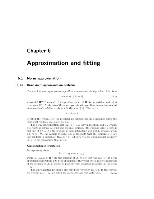
Chapter 6<br />
Approximation and fitting<br />
6.1 Norm approximation<br />
6.1.1 Basic norm approximation problem<br />
The simplest norm approximation problem is an unconstrained problem of the form<br />
minimize ‖Ax − b‖ (6.1)<br />
where A ∈ R m×n and b ∈ R m are problem data, x ∈ R n is the variable, and ‖ · ‖ is<br />
a norm on R m . A solution of the norm approximation problem is sometimes called<br />
an approximate solution of Ax ≈ b, in the norm ‖ · ‖. The vector<br />
r = Ax − b<br />
is called the residual for the problem; its components are sometimes called the<br />
individual residuals associated with x.<br />
The norm approximation problem (6.1) is a convex problem, and is solvable,<br />
i.e., there is always at least one optimal solution. Its optimal value is zero if<br />
and only if b ∈ R(A); the problem is more interesting and useful, however, when<br />
b ∉ R(A). We can assume without loss of generality that the columns of A are<br />
independent; in particular, that m ≥ n. When m = n the optimal point is simply<br />
A −1 b, so we can assume that m > n.<br />
Approximation interpretation<br />
By expressing Ax as<br />
Ax = x 1 a 1 + · · · + x n a n ,<br />
where a 1 , . . . , a n ∈ R m are the columns of A, we see that the goal of the norm<br />
approximation problem is to fit or approximate the vector b by a linear combination<br />
of the columns of A, as closely as possible, with deviation measured in the norm<br />
‖ · ‖.<br />
The approximation problem is also called the regression problem. In this context<br />
the vectors a 1 , . . . , a n are called the regressors, and the vector x 1 a 1 + · · · + x n a n ,
292 6 Approximation and fitting<br />
where x is an optimal solution of the problem, is called the regression of b (onto<br />
the regressors).<br />
Estimation interpretation<br />
A closely related interpretation of the norm approximation problem arises in the<br />
problem of estimating a parameter vector on the basis of an imperfect linear vector<br />
measurement. We consider a linear measurement model<br />
y = Ax + v,<br />
where y ∈ R m is a vector measurement, x ∈ R n is a vector of parameters to be<br />
estimated, and v ∈ R m is some measurement error that is unknown, but presumed<br />
to be small (in the norm ‖ · ‖). The estimation problem is to make a sensible guess<br />
as to what x is, given y.<br />
If we guess that x has the value ˆx, then we are implicitly making the guess that<br />
v has the value y − Aˆx. Assuming that smaller values of v (measured by ‖ · ‖) are<br />
more plausible than larger values, the most plausible guess for x is<br />
ˆx = argmin z ‖Az − y‖.<br />
(These ideas can be expressed more formally in a statistical framework; see chapter<br />
7.)<br />
Geometric interpretation<br />
We consider the subspace A = R(A) ⊆ R m , and a point b ∈ R m . A projection of<br />
the point b onto the subspace A, in the norm ‖ · ‖, is any point in A that is closest<br />
to b, i.e., any optimal point for the problem<br />
minimize ‖u − b‖<br />
subject to u ∈ A.<br />
Parametrizing an arbitrary element of R(A) as u = Ax, we see that solving the<br />
norm approximation problem (6.1) is equivalent to computing a projection of b<br />
onto A.<br />
Design interpretation<br />
We can interpret the norm approximation problem (6.1) as a problem of optimal<br />
design. The n variables x 1 , . . . , x n are design variables whose values are to be<br />
determined. The vector y = Ax gives a vector of m results, which we assume to<br />
be linear functions of the design variables x. The vector b is a vector of target or<br />
desired results. The goal is choose a vector of design variables that achieves, as<br />
closely as possible, the desired results, i.e., Ax ≈ b. We can interpret the residual<br />
vector r as the deviation between the actual results (i.e., Ax) and the desired<br />
or target results (i.e., b). If we measure the quality of a design by the norm of<br />
the deviation between the actual results and the desired results, then the norm<br />
approximation problem (6.1) is the problem of finding the best design.
6.1 Norm approximation 293<br />
Weighted norm approximation problems<br />
An extension of the norm approximation problem is the weighted norm approximation<br />
problem<br />
minimize ‖W (Ax − b)‖<br />
where the problem data W ∈ R m×m is called the weighting matrix. The weighting<br />
matrix is often diagonal, in which case it gives different relative emphasis to<br />
different components of the residual vector r = Ax − b.<br />
The weighted norm problem can be considered as a norm approximation problem<br />
with norm ‖·‖, and data à = W A, ˜b = W b, and therefore treated as a standard<br />
norm approximation problem (6.1). Alternatively, the weighted norm approximation<br />
problem can be considered a norm approximation problem with data A and<br />
b, and the W -weighted norm defined by<br />
(assuming here that W is nonsingular).<br />
Least-squares approximation<br />
‖z‖ W = ‖W z‖<br />
The most common norm approximation problem involves the Euclidean or l 2 -<br />
norm. By squaring the objective, we obtain an equivalent problem which is called<br />
the least-squares approximation problem,<br />
minimize ‖Ax − b‖ 2 2 = r 2 1 + r 2 2 + · · · + r 2 m,<br />
where the objective is the sum of squares of the residuals. This problem can be<br />
solved analytically by expressing the objective as the convex quadratic function<br />
A point x minimizes f if and only if<br />
f(x) = x T A T Ax − 2b T Ax + b T b.<br />
∇f(x) = 2A T Ax − 2A T b = 0,<br />
i.e., if and only if x satisfies the so-called normal equations<br />
A T Ax = A T b,<br />
which always have a solution. Since we assume the columns of A are independent,<br />
the least-squares approximation problem has the unique solution x = (A T A) −1 A T b.<br />
Chebyshev or minimax approximation<br />
When the l ∞ -norm is used, the norm approximation problem<br />
minimize ‖Ax − b‖ ∞ = max{|r 1 |, . . . , |r m |}<br />
is called the Chebyshev approximation problem, or minimax approximation problem,<br />
since we are to minimize the maximum (absolute value) residual. The Chebyshev<br />
approximation problem can be cast as an LP<br />
with variables x ∈ R n and t ∈ R.<br />
minimize t<br />
subject to −t1 ≼ Ax − b ≼ t1,
294 6 Approximation and fitting<br />
Sum of absolute residuals approximation<br />
When the l 1 -norm is used, the norm approximation problem<br />
minimize ‖Ax − b‖ 1 = |r 1 | + · · · + |r m |<br />
is called the sum of (absolute) residuals approximation problem, or, in the context<br />
of estimation, a robust estimator (for reasons that will be clear soon). Like the<br />
Chebyshev approximation problem, the l 1 -norm approximation problem can be<br />
cast as an LP<br />
minimize 1 T t<br />
subject to −t ≼ Ax − b ≼ t,<br />
with variables x ∈ R n and t ∈ R m .<br />
6.1.2 Penalty function approximation<br />
In l p -norm approximation, for 1 ≤ p < ∞, the objective is<br />
(|r 1 | p + · · · + |r m | p ) 1/p .<br />
As in least-squares problems, we can consider the equivalent problem with objective<br />
|r 1 | p + · · · + |r m | p ,<br />
which is a separable and symmetric function of the residuals. In particular, the<br />
objective depends only on the amplitude distribution of the residuals, i.e., the<br />
residuals in sorted order.<br />
We will consider a useful generalization of the l p -norm approximation problem,<br />
in which the objective depends only on the amplitude distribution of the residuals.<br />
The penalty function approximation problem has the form<br />
minimize φ(r 1 ) + · · · + φ(r m )<br />
subject to r = Ax − b,<br />
(6.2)<br />
where φ : R → R is called the (residual) penalty function. We assume that φ is<br />
convex, so the penalty function approximation problem is a convex optimization<br />
problem. In many cases, the penalty function φ is symmetric, nonnegative, and<br />
satisfies φ(0) = 0, but we will not use these properties in our analysis.<br />
Interpretation<br />
We can interpret the penalty function approximation problem (6.2) as follows. For<br />
the choice x, we obtain the approximation Ax of b, which has the associated residual<br />
vector r. A penalty function assesses a cost or penalty for each component<br />
of residual, given by φ(r i ); the total penalty is the sum of the penalties for each<br />
residual, i.e., φ(r 1 ) + · · · + φ(r m ). Different choices of x lead to different resulting<br />
residuals, and therefore, different total penalties. In the penalty function approximation<br />
problem, we minimize the total penalty incurred by the residuals.
PSfrag replacements<br />
6.1 Norm approximation 295<br />
2<br />
1.5<br />
log barrier<br />
quadratic<br />
φ(u)<br />
1<br />
deadzone-linear<br />
0.5<br />
0<br />
−1.5 −1 −0.5 0 0.5 1 1.5<br />
u<br />
Figure 6.1 Some common penalty functions: the quadratic penalty function<br />
φ(u) = u 2 , the deadzone-linear penalty function with deadzone width a =<br />
1/4, and the log barrier penalty function with limit a = 1.<br />
Example 6.1 Some common penalty functions and associated approximation problems.<br />
• By taking φ(u) = |u| p , where p ≥ 1, the penalty function approximation problem<br />
is equivalent to the l p-norm approximation problem. In particular, the<br />
quadratic penalty function φ(u) = u 2 yields least-squares or Euclidean norm<br />
approximation, and the absolute value penalty function φ(u) = |u| yields l 1-<br />
norm approximation.<br />
• The deadzone-linear penalty function (with deadzone width a > 0) is given by<br />
{<br />
0 |u| ≤ a<br />
φ(u) =<br />
|u| − a |u| > a.<br />
The deadzone-linear function assesses no penalty for residuals smaller than a.<br />
• The log barrier penalty function (with limit a > 0) has the form<br />
{<br />
−a 2 log(1 − (u/a) 2 ) |u| < a<br />
φ(u) =<br />
∞ |u| ≥ a.<br />
The log barrier penalty function assesses an infinite penalty for residuals larger<br />
than a.<br />
A deadzone-linear, log barrier, and quadratic penalty function are plotted in figure<br />
6.1. Note that the log barrier function is very close to the quadratic penalty for<br />
|u/a| ≤ 0.25 (see exercise 6.1).<br />
Scaling the penalty function by a positive number does not affect the solution of<br />
the penalty function approximation problem, since this merely scales the objective
296 6 Approximation and fitting<br />
function. But the shape of the penalty function has a large effect on the solution of<br />
the penalty function approximation problem. Roughly speaking, φ(u) is a measure<br />
of our dislike of a residual of value u. If φ is very small (or even zero) for small<br />
values of u, it means we care very little (or not at all) if residuals have these values.<br />
If φ(u) grows rapidly as u becomes large, it means we have a strong dislike for<br />
large residuals; if φ becomes infinite outside some interval, it means that residuals<br />
outside the interval are unacceptable. This simple interpretation gives insight into<br />
the solution of a penalty function approximation problem, as well as guidelines for<br />
choosing a penalty function.<br />
As an example, let us compare l 1 -norm and l 2 -norm approximation, associated<br />
with the penalty functions φ 1 (u) = |u| and φ 2 (u) = u 2 , respectively. For<br />
|u| = 1, the two penalty functions assign the same penalty. For small u we have<br />
φ 1 (u) ≫ φ 2 (u), so l 1 -norm approximation puts relatively larger emphasis on small<br />
residuals compared to l 2 -norm approximation. For large u we have φ 2 (u) ≫ φ 1 (u),<br />
so l 1 -norm approximation puts less weight on large residuals, compared to l 2 -norm<br />
approximation. This difference in relative weightings for small and large residuals<br />
is reflected in the solutions of the associated approximation problems. The amplitude<br />
distribution of the optimal residual for the l 1 -norm approximation problem<br />
will tend to have more zero and very small residuals, compared to the l 2 -norm approximation<br />
solution. In contrast, the l 2 -norm solution will tend to have relatively<br />
fewer large residuals (since large residuals incur a much larger penalty in l 2 -norm<br />
approximation than in l 1 -norm approximation).<br />
Example<br />
An example will illustrate these ideas. We take a matrix A ∈ R 100×30 and vector<br />
b ∈ R 100 (chosen at random, but the results are typical), and compute the l 1 -norm<br />
and l 2 -norm approximate solutions of Ax ≈ b, as well as the penalty function<br />
approximations with a deadzone-linear penalty (with a = 0.5) and log barrier<br />
penalty (with a = 1). Figure 6.2 shows the four associated penalty functions,<br />
and the amplitude distributions of the optimal residuals for these four penalty<br />
approximations. From the plots of the penalty functions we note that<br />
• The l 1 -norm penalty puts the most weight on small residuals and the least<br />
weight on large residuals.<br />
• The l 2 -norm penalty puts very small weight on small residuals, but strong<br />
weight on large residuals.<br />
• The deadzone-linear penalty function puts no weight on residuals smaller<br />
than 0.5, and relatively little weight on large residuals.<br />
• The log barrier penalty puts weight very much like the l 2 -norm penalty for<br />
small residuals, but puts very strong weight on residuals larger than around<br />
0.8, and infinite weight on residuals larger than 1.<br />
Several features are clear from the amplitude distributions:<br />
• For the l 1 -optimal solution, many residuals are either zero or very small. The<br />
l 1 -optimal solution also has relatively more large residuals.
6.1 Norm approximation 297<br />
PSfrag replacements<br />
40<br />
p = 2<br />
p = 1<br />
0<br />
−2<br />
10<br />
−1<br />
0<br />
1<br />
2<br />
0<br />
−2<br />
−1<br />
0<br />
1<br />
2<br />
Log barrier Deadzone<br />
20<br />
0<br />
−2<br />
10<br />
0<br />
−2<br />
−1<br />
−1<br />
0<br />
0<br />
r<br />
1<br />
1<br />
2<br />
2<br />
Figure 6.2 Histogram of residual amplitudes for four penalty functions, with<br />
the (scaled) penalty functions also shown for reference. For the log barrier<br />
plot, the quadratic penalty is also shown, in dashed curve.
298 PSfrag replacements<br />
6 Approximation and fitting<br />
1.5<br />
1<br />
φ(u)<br />
0.5<br />
0<br />
−1.5 −1 −0.5 0 0.5 1 1.5<br />
u<br />
Figure 6.3 A (nonconvex) penalty function that assesses a fixed penalty to<br />
residuals larger than a threshold (which in this example is one): φ(u) = u 2<br />
if |u| ≤ 1 and φ(u) = 1 if |u| > 1. As a result, penalty approximation with<br />
this function would be relatively insensitive to outliers.<br />
• The l 2 -norm approximation has many modest residuals, and relatively few<br />
larger ones.<br />
• For the deadzone-linear penalty, we see that many residuals have the value<br />
±0.5, right at the edge of the ‘free’ zone, for which no penalty is assessed.<br />
• For the log barrier penalty, we see that no residuals have a magnitude larger<br />
than 1, but otherwise the residual distribution is similar to the residual distribution<br />
for l 2 -norm approximation.<br />
Sensitivity to outliers or large errors<br />
In the estimation or regression context, an outlier is a measurement y i = a T i x + v i<br />
for which the noise v i is relatively large. This is often associated with faulty data<br />
or a flawed measurement. When outliers occur, any estimate of x will be associated<br />
with a residual vector with some large components. Ideally we would like to guess<br />
which measurements are outliers, and either remove them from the estimation<br />
process or greatly lower their weight in forming the estimate. (We cannot, however,<br />
assign zero penalty for very large residuals, because then the optimal point would<br />
likely make all residuals large, which yields a total penalty of zero.) This could be<br />
accomplished using penalty function approximation, with a penalty function such<br />
as<br />
{<br />
u<br />
2<br />
|u| ≤ M<br />
φ(u) =<br />
M 2 (6.3)<br />
|u| > M,<br />
shown in figure 6.3. This penalty function agrees with least-squares for any residual<br />
smaller than M, but puts a fixed weight on any residual larger than M, no matter<br />
how much larger it is. In other words, residuals larger than M are ignored; they<br />
are assumed to be associated with outliers or bad data. Unfortunately, the penalty
PSfrag replacements<br />
6.1 Norm approximation 299<br />
2<br />
1.5<br />
φhub(u)<br />
1<br />
0.5<br />
0<br />
−1.5 −1 −0.5 0 0.5 1 1.5<br />
u<br />
Figure 6.4 The solid line is the robust least-squares or Huber penalty function<br />
φ hub , with M = 1. For |u| ≤ M it is quadratic, and for |u| > M it<br />
grows linearly.<br />
function (6.3) is not convex, and the associated penalty function approximation<br />
problem becomes a hard combinatorial optimization problem.<br />
The sensitivity of a penalty function based estimation method to outliers depends<br />
on the (relative) value of the penalty function for large residuals. If we<br />
restrict ourselves to convex penalty functions (which result in convex optimization<br />
problems), the ones that are least sensitive are those for which φ(u) grows linearly,<br />
i.e., like |u|, for large u. Penalty functions with this property are sometimes called<br />
robust, since the associated penalty function approximation methods are much less<br />
sensitive to outliers or large errors than, for example, least-squares.<br />
One obvious example of a robust penalty function is φ(u) = |u|, corresponding<br />
to l 1 -norm approximation. Another example is the robust least-squares or Huber<br />
penalty function, given by<br />
φ hub (u) =<br />
{<br />
u<br />
2<br />
|u| ≤ M<br />
M(2|u| − M) |u| > M,<br />
(6.4)<br />
shown in figure 6.4. This penalty function agrees with the least-squares penalty<br />
function for residuals smaller than M, and then reverts to l 1 -like linear growth for<br />
larger residuals. The Huber penalty function can be considered a convex approximation<br />
of the outlier penalty function (6.3), in the following sense: They agree<br />
for |u| ≤ M, and for |u| > M, the Huber penalty function is the convex function<br />
closest to the outlier penalty function (6.3).<br />
Example 6.2 Robust regression. Figure 6.5 shows 42 points (t i, y i) in a plane, with<br />
two obvious outliers (one at the upper left, and one at lower right). The dashed line<br />
shows the least-squares approximation of the points by a straight line f(t) = α + βt.<br />
The coefficients α and β are obtained by solving the least-squares problem<br />
minimize<br />
∑ 42<br />
i=1 (yi − α − βti)2 ,
300 6 Approximation and fitting<br />
PSfrag replacements 20<br />
10<br />
f(t)<br />
0<br />
−10<br />
−20<br />
−10 −5 0 5 10<br />
t<br />
Figure 6.5 The 42 circles show points that can be well approximated by<br />
an affine function, except for the two outliers at upper left and lower right.<br />
The dashed line is the least-squares fit of a straight line f(t) = α + βt<br />
to the points, and is rotated away from the main locus of points, toward<br />
the outliers. The solid line shows the robust least-squares fit, obtained by<br />
minimizing Huber’s penalty function with M = 1. This gives a far better fit<br />
to the non-outlier data.<br />
with variables α and β. The least-squares approximation is clearly rotated away from<br />
the main locus of the points, toward the two outliers.<br />
The solid line shows the robust least-squares approximation, obtained by minimizing<br />
the Huber penalty function<br />
∑ 42<br />
minimize φ i=1 hub(y i − α − βt i),<br />
with M = 1. This approximation is far less affected by the outliers.<br />
Since l 1 -norm approximation is among the (convex) penalty function approximation<br />
methods that are most robust to outliers, l 1 -norm approximation is sometimes<br />
called robust estimation or robust regression. The robustness property of<br />
l 1 -norm estimation can also be understood in a statistical framework; see page 353.<br />
Small residuals and l 1 -norm approximation<br />
We can also focus on small residuals. Least-squares approximation puts very small<br />
weight on small residuals, since φ(u) = u 2 is very small when u is small. Penalty<br />
functions such as the deadzone-linear penalty function put zero weight on small<br />
residuals. For penalty functions that are very small for small residuals, we expect<br />
the optimal residuals to be small, but not very small. Roughly speaking, there is<br />
little or no incentive to drive small residuals smaller.<br />
In contrast, penalty functions that put relatively large weight on small residuals,<br />
such as φ(u) = |u|, corresponding to l 1 -norm approximation, tend to produce
6.1 Norm approximation 301<br />
optimal residuals many of which are very small, or even exactly zero. This means<br />
that in l 1 -norm approximation, we typically find that many of the equations are<br />
satisfied exactly, i.e., we have a T i x = b i for many i. This phenomenon can be seen<br />
in figure 6.2.<br />
6.1.3 Approximation with constraints<br />
It is possible to add constraints to the basic norm approximation problem (6.1).<br />
When these constraints are convex, the resulting problem is convex. Constraints<br />
arise for a variety of reasons.<br />
• In an approximation problem, constraints can be used to rule out certain unacceptable<br />
approximations of the vector b, or to ensure that the approximator<br />
Ax satisfies certain properties.<br />
• In an estimation problem, the constraints arise as prior knowledge of the<br />
vector x to be estimated, or from prior knowledge of the estimation error v.<br />
• Constraints arise in a geometric setting in determining the projection of a<br />
point b on a set more complicated than a subspace, for example, a cone or<br />
polyhedron.<br />
Some examples will make these clear.<br />
Nonnegativity constraints on variables<br />
We can add the constraint x ≽ 0 to the basic norm approximation problem:<br />
minimize ‖Ax − b‖<br />
subject to x ≽ 0.<br />
In an estimation setting, nonnegativity constraints arise when we estimate a vector<br />
x of parameters known to be nonnegative, e.g., powers, intensities, or rates. The<br />
geometric interpretation is that we are determining the projection of a vector b onto<br />
the cone generated by the columns of A. We can also interpret this problem as<br />
approximating b using a nonnegative linear (i.e., conic) combination of the columns<br />
of A.<br />
Variable bounds<br />
Here we add the constraint l ≼ x ≼ u, where l, u ∈ R n are problem parameters:<br />
minimize ‖Ax − b‖<br />
subject to l ≼ x ≼ u.<br />
In an estimation setting, variable bounds arise as prior knowledge of intervals in<br />
which each variable lies. The geometric interpretation is that we are determining<br />
the projection of a vector b onto the image of a box under the linear mapping<br />
induced by A.
302 6 Approximation and fitting<br />
Probability distribution<br />
We can impose the constraint that x satisfy x ≽ 0, 1 T x = 1:<br />
minimize ‖Ax − b‖<br />
subject to x ≽ 0, 1 T x = 1.<br />
This would arise in the estimation of proportions or relative frequencies, which are<br />
nonnegative and sum to one. It can also be interpreted as approximating b by a<br />
convex combination of the columns of A. (We will have much more to say about<br />
estimating probabilities in §7.2.)<br />
Norm ball constraint<br />
We can add to the basic norm approximation problem the constraint that x lie in<br />
a norm ball:<br />
minimize ‖Ax − b‖<br />
subject to ‖x − x 0 ‖ ≤ d,<br />
where x 0 and d are problem parameters. Such a constraint can be added for several<br />
reasons.<br />
• In an estimation setting, x 0 is a prior guess of what the parameter x is, and d<br />
is the maximum plausible deviation of our estimate from our prior guess. Our<br />
estimate of the parameter x is the value ˆx which best matches the measured<br />
data (i.e., minimizes ‖Az − b‖) among all plausible candidates (i.e., z that<br />
satisfy ‖z − x 0 ‖ ≤ d).<br />
• The constraint ‖x−x 0 ‖ ≤ d can denote a trust region. Here the linear relation<br />
y = Ax is only an approximation of some nonlinear relation y = f(x) that is<br />
valid when x is near some point x 0 , specifically ‖x − x 0 ‖ ≤ d. The problem<br />
is to minimize ‖Ax − b‖ but only over those x for which the model y = Ax is<br />
trusted.<br />
These ideas also come up in the context of regularization; see §6.3.2.<br />
6.2 Least-norm problems<br />
The basic least-norm problem has the form<br />
minimize<br />
subject to<br />
‖x‖<br />
Ax = b<br />
(6.5)<br />
where the data are A ∈ R m×n and b ∈ R m , the variable is x ∈ R n , and ‖ · ‖ is a<br />
norm on R n . A solution of the problem, which always exists if the linear equations<br />
Ax = b have a solution, is called a least-norm solution of Ax = b. The least-norm<br />
problem is, of course, a convex optimization problem.<br />
We can assume without loss of generality that the rows of A are independent, so<br />
m ≤ n. When m = n, the only feasible point is x = A −1 b; the least-norm problem<br />
is interesting only when m < n, i.e., when the equation Ax = b is underdetermined.
6.2 Least-norm problems 303<br />
Reformulation as norm approximation problem<br />
The least-norm problem (6.5) can be formulated as a norm approximation problem<br />
by eliminating the equality constraint. Let x 0 be any solution of Ax = b, and let<br />
Z ∈ R n×k be a matrix whose columns are a basis for the nullspace of A. The<br />
general solution of Ax = b can then be expressed as x 0 + Zu where u ∈ R k . The<br />
least-norm problem (6.5) can be expressed as<br />
minimize<br />
‖x 0 + Zu‖,<br />
with variable u ∈ R k , which is a norm approximation problem. In particular,<br />
our analysis and discussion of norm approximation problems applies to least-norm<br />
problems as well (when interpreted correctly).<br />
Control or design interpretation<br />
We can interpret the least-norm problem (6.5) as a problem of optimal design or<br />
optimal control. The n variables x 1 , . . . , x n are design variables whose values are<br />
to be determined. In a control setting, the variables x 1 , . . . , x n represent inputs,<br />
whose values we are to choose. The vector y = Ax gives m attributes or results of<br />
the design x, which we assume to be linear functions of the design variables x. The<br />
m < n equations Ax = b represent m specifications or requirements on the design.<br />
Since m < n, the design is underspecified; there are n − m degrees of freedom in<br />
the design (assuming A is rank m).<br />
Among all the designs that satisfy the specifications, the least-norm problem<br />
chooses the smallest design, as measured by the norm ‖ · ‖. This can be thought of<br />
as the most efficient design, in the sense that it achieves the specifications Ax = b,<br />
with the smallest possible x.<br />
Estimation interpretation<br />
We assume that x is a vector of parameters to be estimated. We have m < n<br />
perfect (noise free) linear measurements, given by Ax = b. Since we have fewer<br />
measurements than parameters to estimate, our measurements do not completely<br />
determine x. Any parameter vector x that satisfies Ax = b is consistent with our<br />
measurements.<br />
To make a good guess about what x is, without taking further measurements,<br />
we must use prior information. Suppose our prior information, or assumption, is<br />
that x is more likely to be small (as measured by ‖ · ‖) than large. The least-norm<br />
problem chooses as our estimate of the parameter vector x the one that is smallest<br />
(hence, most plausible) among all parameter vectors that are consistent with the<br />
measurements Ax = b. (For a statistical interpretation of the least-norm problem,<br />
see page 359.)<br />
Geometric interpretation<br />
We can also give a simple geometric interpretation of the least-norm problem (6.5).<br />
The feasible set {x | Ax = b} is affine, and the objective is the distance (measured<br />
by the norm ‖ · ‖) between x and the point 0. The least-norm problem finds the
304 6 Approximation and fitting<br />
point in the affine set with minimum distance to 0, i.e., it determines the projection<br />
of the point 0 on the affine set {x | Ax = b}.<br />
Least-squares solution of linear equations<br />
The most common least-norm problem involves the Euclidean or l 2 -norm.<br />
squaring the objective we obtain the equivalent problem<br />
By<br />
minimize ‖x‖ 2 2<br />
subject to Ax = b,<br />
the unique solution of which is called the least-squares solution of the equations<br />
Ax = b. Like the least-squares approximation problem, this problem can be solved<br />
analytically. Introducing the dual variable ν ∈ R m , the optimality conditions are<br />
2x ⋆ + A T ν ⋆ = 0, Ax ⋆ = b,<br />
which is a pair of linear equations, and readily solved. From the first equation<br />
we obtain x ⋆ = −(1/2)A T ν ⋆ ; substituting this into the second equation we obtain<br />
−(1/2)AA T ν ⋆ = b, and conclude<br />
ν ⋆ = −2(AA T ) −1 b, x ⋆ = A T (AA T ) −1 b.<br />
(Since rank A = m < n, the matrix AA T is invertible.)<br />
Least-penalty problems<br />
A useful variation on the least-norm problem (6.5) is the least-penalty problem<br />
minimize φ(x 1 ) + · · · + φ(x n )<br />
subject to Ax = b,<br />
(6.6)<br />
where φ : R → R is convex, nonnegative, and satisfies φ(0) = 0. The penalty<br />
function value φ(u) quantifies our dislike of a component of x having value u;<br />
the least-penalty problem then finds x that has least total penalty, subject to the<br />
constraint Ax = b.<br />
All of the discussion and interpretation of penalty functions in penalty function<br />
approximation can be transposed to the least-penalty problem, by substituting<br />
the amplitude distribution of x (in the least-penalty problem) for the amplitude<br />
distribution of the residual r (in the penalty approximation problem).<br />
Sparse solutions via least l 1 -norm<br />
Recall from the discussion on page 300 that l 1 -norm approximation gives relatively<br />
large weight to small residuals, and therefore results in many optimal residuals<br />
small, or even zero. A similar effect occurs in the least-norm context. The least<br />
l 1 -norm problem,<br />
minimize ‖x‖ 1<br />
subject to Ax = b,<br />
tends to produce a solution x with a large number of components equal to zero.<br />
In other words, the least l 1 -norm problem tends to produce sparse solutions of<br />
Ax = b, often with m nonzero components.
6.3 Regularized approximation 305<br />
It is easy to find solutions of Ax = b that have only m nonzero components.<br />
Choose any set of m indices (out of 1, . . . , n) which are to be the nonzero components<br />
of x. The equation Ax = b reduces to Øx = b, where à is the m × m<br />
submatrix of A obtained by selecting only the chosen columns, and ˜x ∈ R m is the<br />
subvector of x containing the m selected components. If à is nonsingular, then<br />
we can take ˜x = Ã−1 b, which gives a feasible solution x with m or less nonzero<br />
components. If à is singular and b ∉ R(Ã), the equation Øx = b is unsolvable,<br />
which means there is no feasible x with the chosen set of nonzero components. If<br />
à is singular and b ∈ R(Ã), there is a feasible solution with fewer than m nonzero<br />
components.<br />
This approach can be used to find the smallest x with m (or fewer) nonzero<br />
entries, but in general requires examining and comparing all n!/(m!(n−m)!) choices<br />
of m nonzero coefficients of the n coefficients in x. Solving the least l 1 -norm<br />
problem, on the other hand, gives a good heuristic for finding a sparse, and small,<br />
solution of Ax = b.<br />
6.3 Regularized approximation<br />
6.3.1 Bi-criterion formulation<br />
In the basic form of regularized approximation, the goal is to find a vector x that<br />
is small (if possible), and also makes the residual Ax − b small. This is naturally<br />
described as a (convex) vector optimization problem with two objectives, ‖Ax − b‖<br />
and ‖x‖:<br />
minimize (w.r.t. R 2 +) (‖Ax − b‖, ‖x‖) . (6.7)<br />
The two norms can be different: the first, used to measure the size of the residual,<br />
is on R m ; the second, used to measure the size of x, is on R n .<br />
The optimal trade-off between the two objectives can be found using several<br />
methods. The optimal trade-off curve of ‖Ax − b‖ versus ‖x‖, which shows how<br />
large one of the objectives must be made to have the other one small, can then be<br />
plotted. One endpoint of the optimal trade-off curve between ‖Ax − b‖ and ‖x‖<br />
is easy to describe. The minimum value of ‖x‖ is zero, and is achieved only when<br />
x = 0. For this value of x, the residual norm has the value ‖b‖.<br />
The other endpoint of the trade-off curve is more complicated to describe. Let<br />
C denote the set of minimizers of ‖Ax − b‖ (with no constraint on ‖x‖). Then any<br />
minimum norm point in C is Pareto optimal, corresponding to the other endpoint<br />
of the trade-off curve. In other words, Pareto optimal points at this endpoint are<br />
given by minimum norm minimizers of ‖Ax − b‖. If both norms are Euclidean, this<br />
Pareto optimal point is unique, and given by x = A † b, where A † is the pseudoinverse<br />
of A. (See §4.7.6, page 184, and §A.5.4.)
306 6 Approximation and fitting<br />
6.3.2 Regularization<br />
Regularization is a common scalarization method used to solve the bi-criterion<br />
problem (6.7). One form of regularization is to minimize the weighted sum of the<br />
objectives:<br />
minimize ‖Ax − b‖ + γ‖x‖, (6.8)<br />
where γ > 0 is a problem parameter. As γ varies over (0, ∞), the solution of (6.8)<br />
traces out the optimal trade-off curve.<br />
Another common method of regularization, especially when the Euclidean norm<br />
is used, is to minimize the weighted sum of squared norms, i.e.,<br />
minimize ‖Ax − b‖ 2 + δ‖x‖ 2 , (6.9)<br />
for a variety of values of δ > 0.<br />
These regularized approximation problems each solve the bi-criterion problem<br />
of making both ‖Ax − b‖ and ‖x‖ small, by adding an extra term or penalty<br />
associated with the norm of x.<br />
Interpretations<br />
Regularization is used in several contexts. In an estimation setting, the extra term<br />
penalizing large ‖x‖ can be interpreted as our prior knowledge that ‖x‖ is not too<br />
large. In an optimal design setting, the extra term adds the cost of using large<br />
values of the design variables to the cost of missing the target specifications.<br />
The constraint that ‖x‖ be small can also reflect a modeling issue. It might be,<br />
for example, that y = Ax is only a good approximation of the true relationship<br />
y = f(x) between x and y. In order to have f(x) ≈ b, we want Ax ≈ b, and also<br />
need x small in order to ensure that f(x) ≈ Ax.<br />
We will see in §6.4.1 and §6.4.2 that regularization can be used to take into<br />
account variation in the matrix A. Roughly speaking, a large x is one for which<br />
variation in A causes large variation in Ax, and hence should be avoided.<br />
Regularization is also used when the matrix A is square, and the goal is to<br />
solve the linear equations Ax = b. In cases where A is poorly conditioned, or even<br />
singular, regularization gives a compromise between solving the equations (i.e.,<br />
making ‖Ax − b‖ zero) and keeping x of reasonable size.<br />
Regularization comes up in a statistical setting; see §7.1.2.<br />
Tikhonov regularization<br />
The most common form of regularization is based on (6.9), with Euclidean norms,<br />
which results in a (convex) quadratic optimization problem:<br />
minimize ‖Ax − b‖ 2 2 + δ‖x‖ 2 2 = x T (A T A + δI)x − 2b T Ax + b T b. (6.10)<br />
This Tikhonov regularization problem has the analytical solution<br />
x = (A T A + δI) −1 A T b.<br />
Since A T A + δI ≻ 0 for any δ > 0, the Tikhonov regularized least-squares solution<br />
requires no rank (or dimension) assumptions on the matrix A.
6.3 Regularized approximation 307<br />
Smoothing regularization<br />
The idea of regularization, i.e., adding to the objective a term that penalizes large<br />
x, can be extended in several ways. In one useful extension we add a regularization<br />
term of the form ‖Dx‖, in place of ‖x‖. In many applications, the matrix D<br />
represents an approximate differentiation or second-order differentiation operator,<br />
so ‖Dx‖ represents a measure of the variation or smoothness of x.<br />
For example, suppose that the vector x ∈ R n represents the value of some<br />
continuous physical parameter, say, temperature, along the interval [0, 1]: x i is<br />
the temperature at the point i/n. A simple approximation of the gradient or<br />
first derivative of the parameter near i/n is given by n(x i+1 − x i ), and a simple<br />
approximation of its second derivative is given by the second difference<br />
n (n(x i+1 − x i ) − n(x i − x i−1 )) = n 2 (x i+1 − 2x i + x i−1 ).<br />
If ∆ is the (tridiagonal, Toeplitz) matrix<br />
⎡<br />
⎤<br />
1 −2 1 0 · · · 0 0 0 0<br />
0 1 −2 1 · · · 0 0 0 0<br />
0 0 1 −2 · · · 0 0 0 0<br />
∆ = n 2 . . . . . . . .<br />
∈ R (n−2)×n ,<br />
⎢ 0 0 0 0 · · · −2 1 0 0<br />
⎥<br />
⎣ 0 0 0 0 · · · 1 −2 1 0 ⎦<br />
0 0 0 0 · · · 0 1 −2 1<br />
then ∆x represents an approximation of the second derivative of the parameter, so<br />
‖∆x‖ 2 2 represents a measure of the mean-square curvature of the parameter over<br />
the interval [0, 1].<br />
The Tikhonov regularized problem<br />
minimize ‖Ax − b‖ 2 2 + δ‖∆x‖ 2 2<br />
can be used to trade off the objective ‖Ax − b‖ 2 , which might represent a measure<br />
of fit, or consistency with experimental data, and the objective ‖∆x‖ 2 , which is<br />
(approximately) the mean-square curvature of the underlying physical parameter.<br />
The parameter δ is used to control the amount of regularization required, or to<br />
plot the optimal trade-off curve of fit versus smoothness.<br />
We can also add several regularization terms. For example, we can add terms<br />
associated with smoothness and size, as in<br />
minimize ‖Ax − b‖ 2 2 + δ‖∆x‖ 2 2 + η‖x‖ 2 2.<br />
Here, the parameter δ ≥ 0 is used to control the smoothness of the approximate<br />
solution, and the parameter η ≥ 0 is used to control its size.<br />
Example 6.3 Optimal input design. We consider a dynamical system with scalar<br />
input sequence u(0), u(1), . . . , u(N), and scalar output sequence y(0), y(1), . . . , y(N),<br />
related by convolution:<br />
t∑<br />
y(t) = h(τ)u(t − τ), t = 0, 1, . . . , N.<br />
τ=0
308 6 Approximation and fitting<br />
The sequence h(0), h(1), . . . , h(N) is called the convolution kernel or impulse response<br />
of the system.<br />
Our goal is to choose the input sequence u to achieve several goals.<br />
• Output tracking. The primary goal is that the output y should track, or follow,<br />
a desired target or reference signal y des . We measure output tracking error by<br />
the quadratic function<br />
J track = 1<br />
N + 1<br />
N∑<br />
(y(t) − y des (t)) 2 .<br />
t=0<br />
• Small input. The input should not be large. We measure the magnitude of the<br />
input by the quadratic function<br />
J mag = 1<br />
N + 1<br />
N∑<br />
u(t) 2 .<br />
• Small input variations. The input should not vary rapidly. We measure the<br />
magnitude of the input variations by the quadratic function<br />
By minimizing a weighted sum<br />
t=0<br />
J der = 1 N−1<br />
∑<br />
(u(t + 1) − u(t)) 2 .<br />
N<br />
t=0<br />
J track + δJ der + ηJ mag,<br />
where δ > 0 and η > 0, we can trade off the three objectives.<br />
Now we consider a specific example, with N = 200, and impulse response<br />
h(t) = 1 9 (0.9)t (1 − 0.4 cos(2t)).<br />
Figure 6.6 shows the optimal input, and corresponding output (along with the desired<br />
trajectory y des ), for three values of the regularization parameters δ and η. The top<br />
row shows the optimal input and corresponding output for δ = 0, η = 0.005. In this<br />
case we have some regularization for the magnitude of the input, but no regularization<br />
for its variation. While the tracking is good (i.e., we have J track is small), the input<br />
required is large, and rapidly varying. The second row corresponds to δ = 0, η = 0.05.<br />
In this case we have more magnitude regularization, but still no regularization for<br />
variation in u. The corresponding input is indeed smaller, at the cost of a larger<br />
tracking error. The bottom row shows the results for δ = 0.3, η = 0.05. In this<br />
case we have added some regularization for the variation. The input variation is<br />
substantially reduced, with not much increase in output tracking error.<br />
l 1 -norm regularization<br />
Regularization with an l 1 -norm can be used as a heuristic for finding a sparse<br />
solution. For example, consider the problem<br />
minimize ‖Ax − b‖ 2 + γ‖x‖ 1 , (6.11)
6.3 Regularized approximation 309<br />
PSfrag replacements<br />
5<br />
PSfrag replacements<br />
1<br />
0<br />
0.5<br />
u(t)<br />
y(t)<br />
0<br />
−5<br />
−0.5<br />
−1<br />
−10<br />
PSfrag replacements 0 50 100PSfrag150 replacements 200 0 50 100 150 200<br />
t<br />
t<br />
4<br />
1<br />
2<br />
0.5<br />
u(t)<br />
0<br />
y(t)<br />
0<br />
−2<br />
−0.5<br />
−1<br />
−4<br />
PSfrag replacements 0 50 100PSfrag150 replacements 200 0 50 100 150 200<br />
t<br />
t<br />
4<br />
1<br />
2<br />
0.5<br />
u(t)<br />
0<br />
y(t)<br />
0<br />
−2<br />
−0.5<br />
−4<br />
0 50 100 150 200<br />
t<br />
−1<br />
0 50 100<br />
t<br />
150 200<br />
Figure 6.6 Optimal inputs (left) and resulting outputs (right) for three values<br />
of the regularization parameters δ (which corresponds to input variation) and<br />
η (which corresponds to input magnitude). The dashed line in the righthand<br />
plots shows the desired output y des . Top row: δ = 0, η = 0.005; middle row:<br />
δ = 0, η = 0.05; bottom row: δ = 0.3, η = 0.05.
310 6 Approximation and fitting<br />
in which the residual is measured with the Euclidean norm and the regularization is<br />
done with an l 1 -norm. By varying the parameter γ we can sweep out the optimal<br />
trade-off curve between ‖Ax − b‖ 2 and ‖x‖ 1 , which serves as an approximation<br />
of the optimal trade-off curve between ‖Ax − b‖ 2 and the sparsity or cardinality<br />
card(x) of the vector x, i.e., the number of nonzero elements. The problem (6.11)<br />
can be recast and solved as an SOCP.<br />
Example 6.4 Regressor selection problem. We are given a matrix A ∈ R n×m ,<br />
whose columns are potential regressors, and a vector b ∈ R n that is to be fit by a<br />
linear combination of k < m columns of A. The problem is to choose the subset of<br />
k regressors to be used, and the associated coefficients. We can express this problem<br />
as<br />
minimize ‖Ax − b‖ 2<br />
subject to card(x) ≤ k.<br />
In general, this is a hard combinatorial problem.<br />
One straightforward approach is to check every possible sparsity pattern in x with k<br />
nonzero entries. For a fixed sparsity pattern, we can find the optimal x by solving<br />
a least-squares problem, i.e., minimizing ‖Øx − b‖2, where à denotes the submatrix<br />
of A obtained by keeping the columns corresponding to the sparsity pattern, and<br />
˜x is the subvector with the nonzero components of x. This is done for each of the<br />
n!/(k!(n − k)!) sparsity patterns with k nonzeros.<br />
A good heuristic approach is to solve the problem (6.11) for different values of γ,<br />
finding the smallest value of γ that results in a solution with card(x) = k. We then<br />
fix this sparsity pattern and find the value of x that minimizes ‖Ax − b‖ 2.<br />
Figure 6.7 illustrates a numerical example with A ∈ R 10×20 , x ∈ R 20 , b ∈ R 10 . The<br />
circles on the dashed curve are the (globally) Pareto optimal values for the trade-off<br />
between card(x) (vertical axis) and the residual ‖Ax − b‖ 2 (horizontal axis). For<br />
each k, the Pareto optimal point was obtained by enumerating all possible sparsity<br />
patterns with k nonzero entries, as described above. The circles on the solid curve<br />
were obtained with the heuristic approach, by using the sparsity patterns of the<br />
solutions of problem (6.11) for different values of γ. Note that for card(x) = 1, the<br />
heuristic method actually finds the global optimum.<br />
This idea will come up again in basis pursuit (§6.5.4).<br />
6.3.3 Reconstruction, smoothing, and de-noising<br />
In this section we describe an important special case of the bi-criterion approximation<br />
problem described above, and give some examples showing how different<br />
regularization methods perform. In reconstruction problems, we start with a signal<br />
represented by a vector x ∈ R n . The coefficients x i correspond to the value of<br />
some function of time, evaluated (or sampled, in the language of signal processing)<br />
at evenly spaced points. It is usually assumed that the signal does not vary too<br />
rapidly, which means that usually, we have x i ≈ x i+1 . (In this section we consider<br />
signals in one dimension, e.g., audio signals, but the same ideas can be applied to<br />
signals in two or more dimensions, e.g., images or video.)
6.3 Regularized approximation 311<br />
PSfrag replacements<br />
10<br />
8<br />
card(x)<br />
6<br />
4<br />
2<br />
0<br />
0 1 2 3 4<br />
‖Ax − b‖ 2<br />
Figure 6.7 Sparse regressor selection with a matrix A ∈ R 10×20 . The circles<br />
on the dashed line are the Pareto optimal values for the trade-off between<br />
the residual ‖Ax − b‖ 2 and the number of nonzero elements card(x). The<br />
points indicated by circles on the solid line are obtained via the l 1-norm<br />
regularized heuristic.<br />
The signal x is corrupted by an additive noise v:<br />
x cor = x + v.<br />
The noise can be modeled in many different ways, but here we simply assume that<br />
it is unknown, small, and, unlike the signal, rapidly varying. The goal is to form an<br />
estimate ˆx of the original signal x, given the corrupted signal x cor . This process is<br />
called signal reconstruction (since we are trying to reconstruct the original signal<br />
from the corrupted version) or de-noising (since we are trying to remove the noise<br />
from the corrupted signal). Most reconstruction methods end up performing some<br />
sort of smoothing operation on x cor to produce ˆx, so the process is also called<br />
smoothing.<br />
One simple formulation of the reconstruction problem is the bi-criterion problem<br />
minimize (w.r.t. R 2 +) (‖ˆx − x cor ‖ 2 , φ(ˆx)) , (6.12)<br />
where ˆx is the variable and x cor is a problem parameter. The function φ : R n → R<br />
is convex, and is called the regularization function or smoothing objective. It is<br />
meant to measure the roughness, or lack of smoothness, of the estimate ˆx. The<br />
reconstruction problem (6.12) seeks signals that are close (in l 2 -norm) to the corrupted<br />
signal, and that are smooth, i.e., for which φ(ˆx) is small. The reconstruction<br />
problem (6.12) is a convex bi-criterion problem. We can find the Pareto optimal<br />
points by scalarization, and solving a (scalar) convex optimization problem.
312 6 Approximation and fitting<br />
Quadratic smoothing<br />
The simplest reconstruction method uses the quadratic smoothing function<br />
n−1<br />
∑<br />
φ quad (x) = (x i+1 − x i ) 2 = ‖Dx‖ 2 2,<br />
where D ∈ R (n−1)×n is the bidiagonal matrix<br />
⎡<br />
⎤<br />
−1 1 0 · · · 0 0 0<br />
0 −1 1 · · · 0 0 0<br />
D =<br />
⎢ .<br />
.<br />
.<br />
.<br />
.<br />
.<br />
.<br />
⎥<br />
⎣ 0 0 0 · · · −1 1 0 ⎦<br />
0 0 0 · · · 0 −1 1<br />
i=1<br />
We can obtain the optimal trade-off between ‖ˆx−x cor ‖ 2 and ‖Dˆx‖ 2 by minimizing<br />
‖ˆx − x cor ‖ 2 2 + δ‖Dˆx‖ 2 2,<br />
where δ > 0 parametrizes the optimal trade-off curve. The solution of this quadratic<br />
problem,<br />
ˆx = (I + δD T D) −1 x cor ,<br />
can be computed very efficiently since I + δD T D is tridiagonal; see appendix C.<br />
Quadratic smoothing example<br />
Figure 6.8 shows a signal x ∈ R 4000 (top) and the corrupted signal x cor (bottom).<br />
The optimal trade-off curve between the objectives ‖ˆx−x cor ‖ 2 and ‖Dˆx‖ 2 is shown<br />
in figure 6.9. The extreme point on the left of the trade-off curve corresponds to<br />
ˆx = x cor , and has objective value ‖Dx cor ‖ 2 = 4.4. The extreme point on the right<br />
corresponds to ˆx = 0, for which ‖ˆx − x cor ‖ 2 = ‖x cor ‖ 2 = 16.2. Note the clear knee<br />
in the trade-off curve near ‖ˆx − x cor ‖ 2 ≈ 3.<br />
Figure 6.10 shows three smoothed signals on the optimal trade-off curve, corresponding<br />
to ‖ˆx − x cor ‖ 2 = 8 (top), 3 (middle), and 1 (bottom). Comparing the<br />
reconstructed signals with the original signal x, we see that the best reconstruction<br />
is obtained for ‖ˆx − x cor ‖ 2 = 3, which corresponds to the knee of the trade-off<br />
curve. For higher values of ‖ˆx − x cor ‖ 2 , there is too much smoothing; for smaller<br />
values there is too little smoothing.<br />
Total variation reconstruction<br />
Simple quadratic smoothing works well as a reconstruction method when the original<br />
signal is very smooth, and the noise is rapidly varying. But any rapid variations<br />
in the original signal will, obviously, be attenuated or removed by quadratic<br />
smoothing. In this section we describe a reconstruction method that can remove<br />
much of the noise, while still preserving occasional rapid variations in the original<br />
signal. The method is based on the smoothing function<br />
n−1<br />
∑<br />
φ tv (ˆx) = |ˆx i+1 − ˆx i | = ‖Dˆx‖ 1 ,<br />
i=1
6.3 Regularized approximation 313<br />
0.5<br />
PSfrag replacements<br />
x<br />
0<br />
−0.5<br />
0<br />
1000<br />
2000<br />
3000<br />
4000<br />
0.5<br />
xcor<br />
0<br />
−0.5<br />
0<br />
1000<br />
2000<br />
i<br />
3000<br />
4000<br />
Figure 6.8 Top: the original signal x ∈ R 4000 . Bottom: the corrupted signal<br />
x cor.<br />
PSfrag replacements<br />
4<br />
3<br />
‖Dˆx‖2<br />
2<br />
1<br />
0<br />
0 5 10 15 20<br />
‖ˆx − x cor ‖ 2<br />
Figure 6.9 Optimal trade-off curve between ‖Dˆx‖ 2 and ‖ˆx − x cor‖ 2. The<br />
curve has a clear knee near ‖ˆx − x cor‖ ≈ 3.
314 6 Approximation and fitting<br />
PSfrag replacements 0.5<br />
ˆx<br />
0<br />
−0.5<br />
0<br />
1000<br />
2000<br />
3000<br />
4000<br />
0.5<br />
ˆx<br />
0<br />
−0.5<br />
0<br />
1000<br />
2000<br />
3000<br />
4000<br />
0.5<br />
ˆx<br />
0<br />
−0.5<br />
0<br />
1000<br />
2000<br />
i<br />
3000<br />
4000<br />
Figure 6.10 Three smoothed or reconstructed signals ˆx. The top one corresponds<br />
to ‖ˆx − x cor‖ 2 = 8, the middle one to ‖ˆx − x cor‖ 2 = 3, and the<br />
bottom one to ‖ˆx − x cor‖ 2 = 1.<br />
which is called the total variation of x ∈ R n . Like the quadratic smoothness<br />
measure φ quad , the total variation function assigns large values to rapidly varying<br />
ˆx. The total variation measure, however, assigns relatively less penalty to large<br />
values of |x i+1 − x i |.<br />
Total variation reconstruction example<br />
Figure 6.11 shows a signal x ∈ R 2000 (in the top plot), and the signal corrupted<br />
with noise x cor . The signal is mostly smooth, but has several rapid variations or<br />
jumps in value; the noise is rapidly varying.<br />
We first use quadratic smoothing. Figure 6.12 shows three smoothed signals on<br />
the optimal trade-off curve between ‖Dˆx‖ 2 and ‖ˆx−x cor ‖ 2 . In the first two signals,<br />
the rapid variations in the original signal are also smoothed. In the third signal<br />
the steep edges in the signal are better preserved, but there is still a significant<br />
amount of noise left.<br />
Now we demonstrate total variation reconstruction. Figure 6.13 shows the optimal<br />
trade-off curve between ‖Dˆx‖ 1 and ‖ˆx − x corr ‖ 2 . Figure 6.14 show the reconstructed<br />
signals on the optimal trade-off curve, for ‖Dˆx‖ 1 = 10 (top), ‖Dˆx‖ 1 = 8<br />
(middle), and ‖Dˆx‖ 1 = 5 (bottom). We observe that, unlike quadratic smoothing,<br />
total variation reconstruction preserves the sharp transitions in the signal.
6.3 Regularized approximation 315<br />
x<br />
2<br />
1<br />
0<br />
PSfrag replacements −1<br />
−2<br />
0<br />
500<br />
1000<br />
1500<br />
2000<br />
2<br />
1<br />
xcor<br />
0<br />
−1<br />
−2<br />
0<br />
500<br />
1000<br />
i<br />
1500<br />
2000<br />
Figure 6.11 A signal x ∈ R 2000 , and the corrupted signal x cor ∈ R 2000 . The<br />
noise is rapidly varying, and the signal is mostly smooth, with a few rapid<br />
variations.
316 6 Approximation and fitting<br />
2<br />
ˆxi<br />
0<br />
−2<br />
0<br />
PSfrag replacements 2<br />
500<br />
1000<br />
1500<br />
2000<br />
ˆxi<br />
0<br />
−2<br />
0<br />
2<br />
500<br />
1000<br />
1500<br />
2000<br />
ˆxi<br />
0<br />
−2<br />
0<br />
500<br />
1000<br />
i<br />
1500<br />
2000<br />
Figure 6.12 Three quadratically smoothed signals ˆx. The top one corresponds<br />
to ‖ˆx − x cor‖ 2 = 10, the middle one to ‖ˆx − x cor‖ 2 = 7, and the<br />
bottom one to ‖ˆx − x cor‖ 2 = 4. The top one greatly reduces the noise, but<br />
also excessively smooths out the rapid variations in the signal. The bottom<br />
smoothed signal does not give enough noise reduction, and still smooths out<br />
the rapid variations in the original signal. The middle smoothed signal gives<br />
the best compromise, but still smooths out the rapid variations.<br />
PSfrag replacements<br />
250<br />
200<br />
‖Dˆx‖1<br />
150<br />
100<br />
50<br />
0<br />
0 10 20 30 40 50<br />
‖ˆx − x cor ‖ 2<br />
Figure 6.13 Optimal trade-off curve between ‖Dˆx‖ 1 and ‖ˆx − x cor‖ 2.
6.3 Regularized approximation 317<br />
2<br />
ˆx<br />
0<br />
−2<br />
0<br />
PSfrag replacements 2<br />
500<br />
1000<br />
1500<br />
2000<br />
ˆx<br />
0<br />
−2<br />
0<br />
2<br />
500<br />
1000<br />
1500<br />
2000<br />
ˆx<br />
0<br />
−2<br />
0<br />
500<br />
1000<br />
i<br />
1500<br />
2000<br />
Figure 6.14 Three reconstructed signals ˆx, using total variation reconstruction.<br />
The top one corresponds to ‖Dˆx‖ 1 = 10, the middle one to ‖Dˆx‖ 1 = 8,<br />
and the bottom one to ‖Dˆx‖ 1 = 5. The top one does not give quite enough<br />
noise reduction, while the bottom one eliminates some of the slowly varying<br />
parts of the signal. Note that in total variation reconstruction, unlike<br />
quadratic smoothing, the sharp changes in the signal are preserved.
318 6 Approximation and fitting<br />
6.4 Robust approximation<br />
6.4.1 Stochastic robust approximation<br />
We consider an approximation problem with basic objective ‖Ax−b‖, but also wish<br />
to take into account some uncertainty or possible variation in the data matrix A.<br />
(The same ideas can be extended to handle the case where there is uncertainty in<br />
both A and b.) In this section we consider some statistical models for the variation<br />
in A.<br />
We assume that A is a random variable taking values in R m×n , with mean Ā,<br />
so we can describe A as<br />
A = Ā + U,<br />
where U is a random matrix with zero mean. Here, the constant matrix Ā gives<br />
the average value of A, and U describes its statistical variation.<br />
It is natural to use the expected value of ‖Ax − b‖ as the objective:<br />
minimize E ‖Ax − b‖. (6.13)<br />
We refer to this problem as the stochastic robust approximation problem. It is<br />
always a convex optimization problem, but usually not tractable since in most<br />
cases it is very difficult to evaluate the objective or its derivatives.<br />
One simple case in which the stochastic robust approximation problem (6.13)<br />
can be solved occurs when A assumes only a finite number of values, i.e.,<br />
prob(A = A i ) = p i , i = 1, . . . , k,<br />
where A i ∈ R m×n , 1 T p = 1, p ≽ 0. In this case the problem (6.13) has the form<br />
minimize<br />
p 1 ‖A 1 x − b‖ + · · · + p k ‖A k x − b‖,<br />
which is often called a sum-of-norms problem. It can be expressed as<br />
minimize p T t<br />
subject to ‖A i x − b‖ ≤ t i , i = 1, . . . , k,<br />
where the variables are x ∈ R n and t ∈ R k . If the norm is the Euclidean norm,<br />
this sum-of-norms problem is an SOCP. If the norm is the l 1 - or l ∞ -norm, the<br />
sum-of-norms problem can be expressed as an LP; see exercise 6.8.<br />
Some variations on the statistical robust approximation problem (6.13) are<br />
tractable. As an example, consider the statistical robust least-squares problem<br />
minimize E ‖Ax − b‖ 2 2,<br />
where the norm is the Euclidean norm. We can express the objective as<br />
E ‖Ax − b‖ 2 2 =<br />
E(Āx − b + Ux)T (Āx − b + Ux)<br />
= (Āx − b)T (Āx − b) + E xT U T Ux<br />
= ‖Āx − b‖2 2 + x T P x,
6.4 Robust approximation 319<br />
where P = E U T U. Therefore the statistical robust approximation problem has<br />
the form of a regularized least-squares problem<br />
with solution<br />
minimize ‖Āx − b‖2 2 + ‖P 1/2 x‖ 2 2,<br />
x = (ĀT Ā + P ) −1 Ā T b.<br />
This makes perfect sense: when the matrix A is subject to variation, the vector<br />
Ax will have more variation the larger x is, and Jensen’s inequality tells us that<br />
variation in Ax will increase the average value of ‖Ax − b‖ 2 . So we need to balance<br />
making Āx − b small with the desire for a small x (to keep the variation in Ax<br />
small), which is the essential idea of regularization.<br />
This observation gives us another interpretation of the Tikhonov regularized<br />
least-squares problem (6.10), as a robust least-squares problem, taking into account<br />
possible variation in the matrix A. The solution of the Tikhonov regularized leastsquares<br />
problem (6.10) minimizes E ‖(A + U)x − b‖ 2 , where U ij are zero mean,<br />
uncorrelated random variables, with variance δ (and here, A is deterministic).<br />
6.4.2 Worst-case robust approximation<br />
It is also possible to model the variation in the matrix A using a set-based, worstcase<br />
approach. We describe the uncertainty by a set of possible values for A:<br />
A ∈ A ⊆ R m×n ,<br />
which we assume is nonempty and bounded. We define the associated worst-case<br />
error of a candidate approximate solution x ∈ R n as<br />
e wc (x) = sup{‖Ax − b‖ | A ∈ A},<br />
which is always a convex function of x. The (worst-case) robust approximation<br />
problem is to minimize the worst-case error:<br />
minimize e wc (x) = sup{‖Ax − b‖ | A ∈ A}, (6.14)<br />
where the variable is x, and the problem data are b and the set A. When A is the<br />
singleton A = {A}, the robust approximation problem (6.14) reduces to the basic<br />
norm approximation problem (6.1). The robust approximation problem is always<br />
a convex optimization problem, but its tractability depends on the norm used and<br />
the description of the uncertainty set A.<br />
Example 6.5 Comparison of stochastic and worst-case robust approximation. To<br />
illustrate the difference between the stochastic and worst-case formulations of the<br />
robust approximation problem, we consider the least-squares problem<br />
minimize ‖A(u)x − b‖ 2 2,<br />
where u ∈ R is an uncertain parameter and A(u) = A 0 + uA 1. We consider a<br />
specific instance of the problem, with A(u) ∈ R 20×10 , ‖A 0‖ = 10, ‖A 1‖ = 1, and u
PSfrag replacements<br />
320 6 Approximation and fitting<br />
12<br />
10<br />
8<br />
x nom<br />
r(u)<br />
6<br />
x stoch<br />
4<br />
x wc<br />
2<br />
0<br />
−2 −1 0 1 2<br />
u<br />
Figure 6.15 The residual r(u) = ‖A(u)x − b‖ 2 as a function of the uncertain<br />
parameter u for three approximate solutions x: (1) the nominal<br />
least-squares solution x nom; (2) the solution of the stochastic robust approximation<br />
problem x stoch (assuming u is uniformly distributed on [−1, 1]); and<br />
(3) the solution of the worst-case robust approximation problem x wc, assuming<br />
the parameter u lies in the interval [−1, 1]. The nominal solution<br />
achieves the smallest residual when u = 0, but gives much larger residuals<br />
as u approaches −1 or 1. The worst-case solution has a larger residual when<br />
u = 0, but its residuals do not rise much as the parameter u varies over the<br />
interval [−1, 1].<br />
in the interval [−1, 1]. (So, roughly speaking, the variation in the matrix A is around<br />
±10%.)<br />
We find three approximate solutions:<br />
• Nominal optimal. The optimal solution x nom is found, assuming A(u) has its<br />
nominal value A 0.<br />
• Stochastic robust approximation. We find x stoch , which minimizes E ‖A(u)x −<br />
b‖ 2 2, assuming the parameter u is uniformly distributed on [−1, 1].<br />
• Worst-case robust approximation. We find x wc, which minimizes<br />
sup ‖A(u)x − b‖ 2 = max{‖(A 0 − A 1)x − b‖ 2, ‖(A 0 + A 1)x − b‖ 2}.<br />
−1≤u≤1<br />
For each of these three values of x, we plot the residual r(u) = ‖A(u)x − b‖ 2 as a<br />
function of the uncertain parameter u, in figure 6.15. These plots show how sensitive<br />
an approximate solution can be to variation in the parameter u. The nominal solution<br />
achieves the smallest residual when u = 0, but is quite sensitive to parameter<br />
variation: it gives much larger residuals as u deviates from 0, and approaches −1 or<br />
1. The worst-case solution has a larger residual when u = 0, but its residuals do not<br />
rise much as u varies over the interval [−1, 1]. The stochastic robust approximate<br />
solution is in between.
6.4 Robust approximation 321<br />
The robust approximation problem (6.14) arises in many contexts and applications.<br />
In an estimation setting, the set A gives our uncertainty in the linear relation<br />
between the vector to be estimated and our measurement vector. Sometimes the<br />
noise term v in the model y = Ax + v is called additive noise or additive error,<br />
since it is added to the ‘ideal’ measurement Ax. In contrast, the variation in A is<br />
called multiplicative error, since it multiplies the variable x.<br />
In an optimal design setting, the variation can represent uncertainty (arising in<br />
manufacture, say) of the linear equations that relate the design variables x to the<br />
results vector Ax. The robust approximation problem (6.14) is then interpreted as<br />
the robust design problem: find design variables x that minimize the worst possible<br />
mismatch between Ax and b, over all possible values of A.<br />
Finite set<br />
Here we have A = {A 1 , . . . , A k }, and the robust approximation problem is<br />
minimize<br />
max i=1,...,k ‖A i x − b‖.<br />
This problem is equivalent to the robust approximation problem with the polyhedral<br />
set A = conv{A 1 , . . . , A k }:<br />
minimize sup {‖Ax − b‖ | A ∈ conv{A 1 , . . . , A k }} .<br />
We can cast the problem in epigraph form as<br />
minimize t<br />
subject to ‖A i x − b‖ ≤ t, i = 1, . . . , k,<br />
which can be solved in a variety of ways, depending on the norm used. If the norm<br />
is the Euclidean norm, this is an SOCP. If the norm is the l 1 - or l ∞ -norm, we can<br />
express it as an LP.<br />
Norm bound error<br />
Here the uncertainty set A is a norm ball, A = {Ā + U | ‖U‖ ≤ a}, where ‖ · ‖ is a<br />
norm on R m×n . In this case we have<br />
e wc (x) = sup{‖Āx − b + Ux‖ | ‖U‖ ≤ a},<br />
which must be carefully interpreted since the first norm appearing is on R m (and<br />
is used to measure the size of the residual) and the second one appearing is on<br />
R m×n (used to define the norm ball A).<br />
This expression for e wc (x) can be simplified in several cases. As an example,<br />
let us take the Euclidean norm on R n and the associated induced norm on R m×n ,<br />
i.e., the maximum singular value. If Āx − b ≠ 0 and x ≠ 0, the supremum in the<br />
expression for e wc (x) is attained for U = auv T , with<br />
and the resulting worst-case error is<br />
u = Āx − b<br />
‖Āx − b‖ , v = x ,<br />
2 ‖x‖ 2<br />
e wc (x) = ‖Āx − b‖ 2 + a‖x‖ 2 .
322 6 Approximation and fitting<br />
(It is easily verified that this expression is also valid if x or Āx − b is zero.) The<br />
robust approximation problem (6.14) then becomes<br />
minimize ‖Āx − b‖ 2 + a‖x‖ 2 ,<br />
which is a regularized norm problem, solvable as the SOCP<br />
minimize t 1 + at 2<br />
subject to ‖Āx − b‖ 2 ≤ t 1 , ‖x‖ 2 ≤ t 2 .<br />
Since the solution of this problem is the same as the solution of the regularized<br />
least-squares problem<br />
minimize ‖Āx − b‖2 2 + δ‖x‖ 2 2<br />
for some value of the regularization parameter δ, we have another interpretation of<br />
the regularized least-squares problem as a worst-case robust approximation problem.<br />
Uncertainty ellipsoids<br />
We can also describe the variation in A by giving an ellipsoid of possible values for<br />
each row:<br />
A = {[a 1 · · · a m ] T | a i ∈ E i , i = 1, . . . , m},<br />
where<br />
E i = {ā i + P i u | ‖u‖ 2 ≤ 1}.<br />
The matrix P i ∈ R n×n describes the variation in a i . We allow P i to have a nontrivial<br />
nullspace, in order to model the situation when the variation in a i is restricted<br />
to a subspace. As an extreme case, we take P i = 0 if there is no uncertainty in a i .<br />
With this ellipsoidal uncertainty description, we can give an explicit expression<br />
for the worst-case magnitude of each residual:<br />
sup |a T i x − b i | = sup{|ā T i x − b i + (P i u) T x| | ‖u‖ 2 ≤ 1}<br />
a i∈E i<br />
= |ā T i x − b i | + ‖P T i x‖ 2 .<br />
Using this result we can solve several robust approximation problems.<br />
example, the robust l 2 -norm approximation problem<br />
For<br />
minimize e wc (x) = sup{‖Ax − b‖ 2 | a i ∈ E i , i = 1, . . . , m}<br />
can be reduced to an SOCP, as follows. An explicit expression for the worst-case<br />
error is given by<br />
(<br />
∑ m (<br />
) ) 2 1/2 ( m<br />
) 1/2<br />
∑<br />
e wc (x) = sup |a T i x − b i | = (|ā T i x − b i | + ‖Pi T x‖ 2 ) 2 .<br />
a i∈E i<br />
i=1<br />
To minimize e wc (x) we can solve<br />
i=1<br />
minimize ‖t‖ 2<br />
subject to |ā T i x − b i| + ‖Pi T x‖ 2 ≤ t i , i = 1, . . . , m,
6.4 Robust approximation 323<br />
where we introduced new variables t 1 , . . . , t m . This problem can be formulated as<br />
minimize ‖t‖ 2<br />
subject to ā T i x − b i + ‖Pi T x‖ 2 ≤ t i , i = 1, . . . , m<br />
−ā T i x + b i + ‖Pi T x‖ 2 ≤ t i , i = 1, . . . , m,<br />
which becomes an SOCP when put in epigraph form.<br />
Norm bounded error with linear structure<br />
As a generalization of the norm bound description A = {Ā + U | ‖U‖ ≤ a}, we can<br />
define A as the image of a norm ball under an affine transformation:<br />
A = {Ā + u 1A 1 + u 2 A 2 + · · · + u p A p | ‖u‖ ≤ 1},<br />
where ‖ · ‖ is a norm on R p , and the p + 1 matrices Ā, A 1, . . . , A p ∈ R m×n are<br />
given. The worst-case error can be expressed as<br />
where P and q are defined as<br />
e wc (x) = sup ‖(Ā + u 1A 1 + · · · + u p A p )x − b‖<br />
‖u‖≤1<br />
= sup ‖P (x)u + q(x)‖,<br />
‖u‖≤1<br />
P (x) = [ A 1 x A 2 x · · · A p x ] ∈ R m×p , q(x) = Āx − b ∈ Rm .<br />
As a first example, we consider the robust Chebyshev approximation problem<br />
minimize e wc (x) = sup ‖u‖∞≤1 ‖(Ā + u 1A 1 + · · · + u p A p )x − b‖ ∞ .<br />
In this case we can derive an explicit expression for the worst-case error. Let p i (x) T<br />
denote the ith row of P (x). We have<br />
e wc (x) = sup ‖P (x)u + q(x)‖ ∞<br />
‖u‖ ∞≤1<br />
= max<br />
sup<br />
i=1,...,m ‖u‖ ∞≤1<br />
|p i (x) T u + q i (x)|<br />
= max<br />
i=1,...,m (‖p i(x)‖ 1 + |q i (x)|).<br />
The robust Chebyshev approximation problem can therefore be cast as an LP<br />
minimize t<br />
subject to −y 0 ≼ Āx − b ≼ y 0<br />
−y k ≼ A k x ≼ y k , k = 1, . . . , p<br />
y 0 + ∑ p<br />
k=1 y k ≼ t1,<br />
with variables x ∈ R n , y k ∈ R m , t ∈ R.<br />
As another example, we consider the robust least-squares problem<br />
minimize e wc (x) = sup ‖u‖2≤1 ‖(Ā + u 1A 1 + · · · + u p A p )x − b‖ 2 .
324 6 Approximation and fitting<br />
Here we use Lagrange duality to evaluate e wc . The worst-case error e wc (x) is the<br />
squareroot of the optimal value of the (nonconvex) quadratic optimization problem<br />
maximize ‖P (x)u + q(x)‖ 2 2<br />
subject to u T u ≤ 1,<br />
with u as variable. The Lagrange dual of this problem can be expressed as the<br />
SDP<br />
minimize t<br />
⎡<br />
+ λ<br />
⎤<br />
I P (x) q(x)<br />
subject to ⎣ P (x) T λI 0 ⎦ (6.15)<br />
≽ 0<br />
q(x) T 0 t<br />
with variables t, λ ∈ R. Moreover, as mentioned in §5.2 and §B.1 (and proved<br />
in §B.4), strong duality holds for this pair of primal and dual problems. In other<br />
words, for fixed x, we can compute e wc (x) 2 by solving the SDP (6.15) with variables<br />
t and λ. Optimizing jointly over t, λ, and x is equivalent to minimizing e wc (x) 2 .<br />
We conclude that the robust least-squares problem is equivalent to the SDP (6.15)<br />
with x, λ, t as variables.<br />
Example 6.6 Comparison of worst-case robust, Tikhonov regularized, and nominal<br />
least-squares solutions. We consider an instance of the robust approximation problem<br />
minimize sup ‖u‖2 ≤1 ‖(Ā + u1A1 + u2A2)x − b‖2, (6.16)<br />
with dimensions m = 50, n = 20. The matrix Ā has norm 10, and the two matrices<br />
A 1 and A 2 have norm 1, so the variation in the matrix A is, roughly speaking, around<br />
10%. The uncertainty parameters u 1 and u 2 lie in the unit disk in R 2 .<br />
We compute the optimal solution of the robust least-squares problem (6.16) x rls , as<br />
well as the solution of the nominal least-squares problem x ls (i.e., assuming u = 0),<br />
and also the Tikhonov regularized solution x tik , with δ = 1.<br />
To illustrate the sensitivity of each of these approximate solutions to the parameter<br />
u, we generate 10 5 parameter vectors, uniformly distributed on the unit disk, and<br />
evaluate the residual<br />
‖(A 0 + u 1A 1 + u 2A 2)x − b‖ 2<br />
for each parameter value. The distributions of the residuals are shown in figure 6.16.<br />
We can make several observations. First, the residuals of the nominal least-squares<br />
solution are widely spread, from a smallest value around 0.52 to a largest value<br />
around 4.9. In particular, the least-squares solution is very sensitive to parameter<br />
variation. In contrast, both the robust least-squares and Tikhonov regularized solutions<br />
exhibit far smaller variation in residual as the uncertainty parameter varies<br />
over the unit disk. The robust least-squares solution, for example, achieves a residual<br />
between 2.0 and 2.6 for all parameters in the unit disk.<br />
6.5 Function fitting and interpolation<br />
In function fitting problems, we select a member of a finite-dimensional subspace<br />
of functions that best fits some given data or requirements. For simplicity we
6.5 Function fitting and interpolation 325<br />
PSfrag replacements<br />
0.25<br />
0.2<br />
x rls<br />
frequency<br />
0.15<br />
0.1<br />
0.05<br />
x tik<br />
x ls<br />
0<br />
0 1 2 3 4 5<br />
‖(A 0 + u 1 A 1 + u 2 A 2 )x − b‖ 2<br />
Figure 6.16 Distribution of the residuals for the three solutions of a leastsquares<br />
problem (6.16): x ls , the least-squares solution assuming u = 0; x tik ,<br />
the Tikhonov regularized solution with δ = 1; and x rls , the robust leastsquares<br />
solution. The histograms were obtained by generating 10 5 values of<br />
the uncertain parameter vector u from a uniform distribution on the unit<br />
disk in R 2 . The bins have width 0.1.
326 6 Approximation and fitting<br />
consider real-valued functions; the ideas are readily extended to handle vectorvalued<br />
functions as well.<br />
6.5.1 Function families<br />
We consider a family of functions f 1 , . . . , f n : R k → R, with common domain<br />
dom f i = D. With each x ∈ R n we associate the function f : R k → R given by<br />
f(u) = x 1 f 1 (u) + · · · + x n f n (u) (6.17)<br />
with dom f = D. The family {f 1 , . . . , f n } is sometimes called the set of basis<br />
functions (for the fitting problem) even when the functions are not independent.<br />
The vector x ∈ R n , which parametrizes the subspace of functions, is our optimization<br />
variable, and is sometimes called the coefficient vector. The basis functions<br />
generate a subspace F of functions on D.<br />
In many applications the basis functions are specially chosen, using prior knowledge<br />
or experience, in order to reasonably model functions of interest with the<br />
finite-dimensional subspace of functions. In other cases, more generic function<br />
families are used. We describe a few of these below.<br />
Polynomials<br />
One common subspace of functions on R consists of polynomials of degree less<br />
than n. The simplest basis consists of the powers, i.e., f i (t) = t i−1 , i = 1, . . . , n.<br />
In many applications, the same subspace is described using a different basis, for<br />
example, a set of polynomials f 1 , . . . , f n , of degree less than n, that are orthonormal<br />
with respect to some positive function (or measure) φ : R n → R + , i.e.,<br />
∫<br />
{<br />
1 i = j<br />
f i (t)f j (t)φ(t) dt =<br />
0 i ≠ j.<br />
Another common basis for polynomials is the Lagrange basis f 1 , . . . , f n associated<br />
with distinct points t 1 , . . . , t n , which satisfy<br />
{<br />
1 i = j<br />
f i (t j ) =<br />
0 i ≠ j.<br />
We can also consider polynomials on R k , with a maximum total degree, or a<br />
maximum degree for each variable.<br />
As a related example, we have trigonometric polynomials of degree less than n,<br />
with basis<br />
sin kt, k = 1, . . . , n − 1, cos kt, k = 0, . . . , n − 1.<br />
Piecewise-linear functions<br />
We start with a triangularization of the domain D, which means the following. We<br />
have a set of mesh or grid points g 1 , . . . , g n ∈ R k , and a partition of D into a set<br />
of simplexes:<br />
D = S 1 ∪ · · · ∪ S n , int(S i ∩ S j ) = ∅ for i ≠ j.
6.5 Function fitting and interpolation 327<br />
1<br />
PSfrag replacements<br />
f(u1, u2)<br />
0<br />
0<br />
u 2<br />
1<br />
1<br />
u 1<br />
0<br />
Figure 6.17 A piecewise-linear function of two variables, on the unit square.<br />
The triangulation consists of 98 simplexes, and a uniform grid of 64 points<br />
in the unit square.<br />
Each simplex is the convex hull of k + 1 grid points, and we require that each grid<br />
point is a vertex of any simplex it lies in.<br />
Given a triangularization, we can construct a piecewise-linear linear (or more<br />
precisely, piecewise-affine) function f by assigning function values f(g i ) = x i to the<br />
grid points, and then extending the function affinely on each simplex. The function<br />
f can be expressed as (6.17) where the basis functions f i are affine on each simplex<br />
and are defined by the conditions<br />
f i (g j ) =<br />
{ 1 i = j<br />
0 i ≠ j.<br />
By construction, such a function is continuous.<br />
Figure 6.17 shows an example for k = 2.<br />
Piecewise polynomials and splines<br />
The idea of piecewise-affine functions on a triangulated domain is readily extended<br />
to piecewise polynomials and other functions.<br />
Piecewise polynomials are defined as polynomials (of some maximum degree)<br />
on each simplex of the triangulation, which are continuous, i.e., the polynomials<br />
agree at the boundaries between simplexes. By further restricting the piecewise<br />
polynomials to have continuous derivatives up to a certain order, we can define<br />
various classes of spline functions. Figure 6.18 shows an example of a cubic spline,<br />
i.e., a piecewise polynomial of degree 3 on R, with continuous first and second<br />
derivatives.
328 6 Approximation and fitting<br />
PSfrag replacements<br />
p 2 (u)<br />
p 3 (u)<br />
f(u)<br />
p 1 (u)<br />
u 0 u 1 u 2 u 3<br />
u<br />
Figure 6.18 Cubic spline. A cubic spline is a piecewise polynomial, with<br />
continuous first and second derivatives. In this example, the cubic spline f<br />
is formed from the three cubic polynomials p 1 (on [u 0, u 1]), p 2 (on [u 1, u 2]),<br />
and p 3 (on [u 2, u 3]). Adjacent polynomials have the same function value,<br />
and equal first and second derivatives, at the boundary points u 1 and u 2.<br />
In this example, the dimension of the family of functions is n = 6, since<br />
we have 12 polynomial coefficients (4 per cubic polynomial), and 6 equality<br />
constraints (3 each at u 1 and u 2).
6.5 Function fitting and interpolation 329<br />
6.5.2 Constraints<br />
In this section we describe some constraints that can be imposed on the function<br />
f, and therefore, on the variable x ∈ R n .<br />
Function value interpolation and inequalities<br />
Let v be a point in D. The value of f at v,<br />
f(v) =<br />
n∑<br />
x i f i (v),<br />
i=1<br />
is a linear function of x. Therefore interpolation conditions<br />
f(v j ) = z j , j = 1, . . . , m,<br />
which require the function f to have the values z j ∈ R at specified points v j ∈ D,<br />
form a set of linear equalities in x. More generally, inequalities on the function<br />
value at a given point, as in l ≤ f(v) ≤ u, are linear inequalities on the variable x.<br />
There are many other interesting convex constraints on f (hence, x) that involve<br />
the function values at a finite set of points v 1 , . . . , v N . For example, the Lipschitz<br />
constraint<br />
|f(v j ) − f(v k )| ≤ L‖v j − v k ‖, j, k = 1, . . . , m,<br />
forms a set of linear inequalities in x.<br />
We can also impose inequalities on the function values at an infinite number of<br />
points. As an example, consider the nonnegativity constraint<br />
f(u) ≥ 0 for all u ∈ D.<br />
This is a convex constraint on x (since it is the intersection of an infinite number<br />
of halfspaces), but may not lead to a tractable problem except in special cases<br />
that exploit the particular structure of the functions. One simple example occurs<br />
when the functions are piecewise-linear. In this case, if the function values are<br />
nonnegative at the grid points, the function is nonnegative everywhere, so we obtain<br />
a simple (finite) set of linear inequalities.<br />
As a less trivial example, consider the case when the functions are polynomials<br />
on R, with even maximum degree 2k (i.e., n = 2k + 1), and D = R. As shown in<br />
exercise 2.37, page 65, the nonnegativity constraint<br />
is equivalent to<br />
p(u) = x 1 + x 2 u + · · · + x 2k+1 u 2k ≥ 0 for all u ∈ R,<br />
x i =<br />
∑<br />
m+n=i+1<br />
where Y ∈ S k+1 is an auxiliary variable.<br />
Y mn , i = 1, . . . , 2k + 1, Y ≽ 0,
330 6 Approximation and fitting<br />
Derivative constraints<br />
Suppose the basis functions f i are differentiable at a point v ∈ D. The gradient<br />
∇f(v) =<br />
n∑<br />
x i ∇f i (v),<br />
i=1<br />
is a linear function of x, so interpolation conditions on the derivative of f at v<br />
reduce to linear equality constraints on x. Requiring that the norm of the gradient<br />
at v not exceed a given limit,<br />
n∑<br />
‖∇f(v)‖ =<br />
x<br />
∥ i ∇f i (v)<br />
∥ ≤ M,<br />
i=1<br />
is a convex constraint on x. The same idea extends to higher derivatives. For<br />
example, if f is twice differentiable at v, the requirement that<br />
lI ≼ ∇ 2 f(v) ≼ uI<br />
is a linear matrix inequality in x, hence convex.<br />
We can also impose constraints on the derivatives at an infinite number of<br />
points. For example, we can require that f is monotone:<br />
f(u) ≥ f(v) for all u, v ∈ D, u ≽ v.<br />
This is a convex constraint in x, but may not lead to a tractable problem except in<br />
special cases. When f is piecewise affine, for example, the monotonicity constraint<br />
is equivalent to the condition ∇f(v) ≽ 0 inside each of the simplexes. Since the<br />
gradient is a linear function of the grid point values, this leads to a simple (finite)<br />
set of linear inequalities.<br />
As another example, we can require that the function be convex, i.e., satisfy<br />
f((u + v)/2) ≤ (f(u) + f(v))/2 for all u, v ∈ D<br />
(which is enough to ensure convexity when f is continuous). This is a convex constraint,<br />
which has a tractable representation in some cases. One obvious example<br />
is when f is quadratic, in which case the convexity constraint reduces to the requirement<br />
that the quadratic part of f be nonnegative, which is an LMI. Another<br />
example in which a convexity constraint leads to a tractable problem is described<br />
in more detail in §6.5.5.<br />
Integral constraints<br />
Any linear functional L on the subspace of functions can be expressed as a linear<br />
function of x, i.e., we have L(f) = c T x. Evaluation of f (or a derivative) at a point<br />
is just a special case. As another example, the linear functional<br />
∫<br />
L(f) = φ(u)f(u) du,<br />
D
6.5 Function fitting and interpolation 331<br />
where φ : R k → R, can be expressed as L(f) = c T x, where<br />
∫<br />
c i = φ(u)f i (u) du.<br />
D<br />
Thus, a constraint of the form L(f) = a is a linear equality constraint on x. One<br />
example of such a constraint is the moment constraint<br />
∫<br />
t m f(t) dt = a<br />
(where f : R → R).<br />
D<br />
6.5.3 Fitting and interpolation problems<br />
Minimum norm function fitting<br />
In a fitting problem, we are given data<br />
(u 1 , y 1 ), . . . , (u m , y m )<br />
with u i ∈ D and y i ∈ R, and seek a function f ∈ F that matches this data as<br />
closely as possible. For example in least-squares fitting we consider the problem<br />
minimize<br />
∑ m<br />
i=1 (f(u i) − y i ) 2 ,<br />
which is a simple least-squares problem in the variable x. We can add a variety of<br />
constraints, for example linear inequalities that must be satisfied by f at various<br />
points, constraints on the derivatives of f, monotonicity constraints, or moment<br />
constraints.<br />
Example 6.7 Polynomial fitting. We are given data u 1, . . . , u m ∈ R and v 1, . . . , v m ∈<br />
R, and hope to approximately fit a polynomial of the form<br />
p(u) = x 1 + x 2u + · · · + x nu n−1<br />
to the data. For each x we form the vector of errors,<br />
e = (p(u 1) − v 1, . . . , p(u m) − v m) .<br />
To find the polynomial that minimizes the norm of the error, we solve the norm<br />
approximation problem<br />
minimize<br />
‖e‖ = ‖Ax − v‖<br />
with variable x ∈ R n , where A ij = u j−1<br />
i<br />
, i = 1, . . . , m, j = 1, . . . , n.<br />
Figure 6.19 shows an example with m = 40 data points and n = 6 (i.e., polynomials<br />
of maximum degree 5), for the l 2- and l ∞-norms.
332 6 Approximation and fitting<br />
PSfrag replacements0.2<br />
p(u)<br />
0.1<br />
0<br />
−0.1<br />
−1 −0.5 0 0.5 1<br />
u<br />
Figure 6.19 Two polynomials of degree 5 that approximate the 40 data<br />
points shown as circles. The polynomial shown as a solid line minimizes the<br />
l 2-norm of the error; the polynomial shown as a dashed line minimizes the<br />
l ∞-norm.<br />
PSfrag replacements0.2<br />
f(u)<br />
0.1<br />
0<br />
−0.1<br />
−1 −0.5 0 0.5 1<br />
u<br />
Figure 6.20 Two cubic splines that approximate the 40 data points shown as<br />
circles (which are the same as the data in figure 6.19). The spline shown as<br />
a solid line minimizes the l 2-norm of the error; the spline shown as a dashed<br />
line minimizes the l ∞-norm. As in the polynomial approximation shown in<br />
figure 6.19, the dimension of the subspace of fitting functions is 6.
6.5 Function fitting and interpolation 333<br />
Example 6.8 Spline fitting. Figure 6.20 shows the same data as in example 6.7,<br />
and two optimal fits with cubic splines. The interval [−1, 1] is divided into three<br />
equal intervals, and we consider piecewise polynomials, with maximum degree 3, with<br />
continuous first and second derivatives. The dimension of this subspace of functions<br />
is 6, the same as the dimension of polynomials with maximum degree 5, considered<br />
in example 6.7.<br />
In the simplest forms of function fitting, we have m ≫ n, i.e., the number<br />
of data points is much larger than the dimension of the subspace of functions.<br />
Smoothing is accomplished automatically, since all members of the subspace are<br />
smooth.<br />
Least-norm interpolation<br />
In another variation of function fitting, we have fewer data points than the dimension<br />
of the subspace of functions. In the simplest case, we require that the function<br />
we choose must satisfy the interpolation conditions<br />
f(u i ) = y i , i = 1, . . . , m,<br />
which are linear equality constraints on x. Among the functions that satisfy these<br />
interpolation conditions, we might seek one that is smoothest, or smallest. These<br />
lead to least-norm problems.<br />
In the most general function fitting problem, we can optimize an objective<br />
(such as some measure of the error e), subject to a variety of convex constraints<br />
that represent our prior knowledge of the underlying function.<br />
Interpolation, extrapolation, and bounding<br />
By evaluating the optimal function fit ˆf at a point v not in the original data set,<br />
we obtain a guess of what the value of the underlying function is, at the point v.<br />
This is called interpolation when v is between or near the given data points (e.g.,<br />
v ∈ conv{v 1 , . . . , v m }), and extrapolation otherwise.<br />
We can also produce an interval in which the value f(v) can lie, by maximizing<br />
and minimizing (the linear function) f(v), subject to the constraints. We can use<br />
the function fit to help identify faulty data or outliers. Here we might use, for<br />
example, an l 1 -norm fit, and look for data points with large errors.<br />
6.5.4 Sparse descriptions and basis pursuit<br />
In basis pursuit, there is a very large number of basis functions, and the goal is to<br />
find a good fit of the given data as a linear combination of a small number of the<br />
basis functions. (In this context the function family is linearly dependent, and is<br />
sometimes referred to as an over-complete basis or dictionary.) This is called basis<br />
pursuit since we are selecting a much smaller basis, from the given over-complete<br />
basis, to model the data.
334 6 Approximation and fitting<br />
Thus we seek a function f ∈ F that fits the data well,<br />
f(u i ) ≈ y i , i = 1, . . . , m,<br />
with a sparse coefficient vector x, i.e., card(x) small. In this case we refer to<br />
f = x 1 f 1 + · · · + x n f n = ∑ x i f i ,<br />
i∈B<br />
where B = {i | x i ≠ 0} is the set of indices of the chosen basis elements, as a sparse<br />
description of the data. Mathematically, basis pursuit is the same as the regressor<br />
selection problem (see §6.4), but the interpretation (and scale) of the optimization<br />
problem are different.<br />
Sparse descriptions and basis pursuit have many uses. They can be used for<br />
de-noising or smoothing, or data compression for efficient transmission or storage<br />
of a signal. In data compression, the sender and receiver both know the dictionary,<br />
or basis elements. To send a signal to the receiver, the sender first finds a sparse<br />
representation of the signal, and then sends to the receiver only the nonzero coefficients<br />
(to some precision). Using these coefficients, the receiver can reconstruct<br />
(an approximation of) the original signal.<br />
One common approach to basis pursuit is the same as the method for regressor<br />
selection described in §6.4, and based on l 1 -norm regularization as a heuristic for<br />
finding sparse descriptions. We first solve the convex problem<br />
minimize<br />
∑ m<br />
i=1 (f(u i) − y i )) 2 + γ‖x‖ 1 , (6.18)<br />
where γ > 0 is a parameter used to trade off the quality of the fit to the data,<br />
and the sparsity of the coefficient vector. The solution of this problem can be used<br />
directly, or followed by a refinement step, in which the best fit is found, using the<br />
sparsity pattern of the solution of (6.18). In other words, we first solve (6.18), to<br />
obtain ˆx. We then set B = {i | ˆx i ≠ 0}, i.e., the set of indices corresponding to<br />
nonzero coefficients. Then we solve the least-squares problem<br />
minimize<br />
∑ m<br />
i=1 (f(u i) − y i )) 2<br />
with variables x i , i ∈ B, and x i = 0 for i ∉ B.<br />
In basis pursuit and sparse description applications it is not uncommon to have<br />
a very large dictionary, with n on the order of 10 4 or much more. To be effective,<br />
algorithms for solving (6.18) must exploit problem structure, which derives from<br />
the structure of the dictionary signals.<br />
Time-frequency analysis via basis pursuit<br />
In this section we illustrate basis pursuit and sparse representation with a simple<br />
example. We consider functions (or signals) on R, with the range of interest [0, 1].<br />
We think of the independent variable as time, so we use t (instead of u) to denote<br />
it.<br />
We first describe the basis functions in the dictionary. Each basis function is a<br />
Gaussian sinusoidal pulse, or Gabor function, with form<br />
e −(t−τ)2 /σ 2 cos(ωt + φ),
6.5 Function fitting and interpolation 335<br />
1<br />
f0.5,0,c<br />
0<br />
−1<br />
0<br />
1<br />
0.2<br />
0.4<br />
0.6<br />
0.8<br />
1<br />
f0.5,75,c<br />
0<br />
−1<br />
0<br />
1<br />
0.2<br />
0.4<br />
0.6<br />
0.8<br />
1<br />
f0.5,150,c<br />
0<br />
−1<br />
0<br />
0.2<br />
0.4<br />
Figure 6.21 Three of the basis elements in the dictionary, all with center time<br />
τ = 0.5 and cosine phase. The top signal has frequency ω = 0, the middle<br />
one has frequency ω = 75, and the bottom one has frequency ω = 150.<br />
t<br />
0.6<br />
0.8<br />
1<br />
where σ > 0 gives the width of the pulse, τ is the time of (the center of) the pulse,<br />
ω ≥ 0 is the frequency, and φ is the phase angle. All of the basis functions have<br />
width σ = 0.05. The pulse times and frequencies are<br />
τ = 0.002k, k = 0, . . . , 500, ω = 5k, k = 0, . . . , 30.<br />
For each time τ, there is one basis element with frequency zero (and phase φ = 0),<br />
and 2 basis elements (cosine and sine, i.e., phase φ = 0 and φ = π/2) for each of 30<br />
remaining frequencies, so all together there are 501 × 61 = 30561 basis elements.<br />
The basis elements are naturally indexed by time, frequency, and phase (cosine or<br />
sine), so we denote them as<br />
f τ,ω,c , τ = 0, 0.002, . . . , 1, ω = 0, 5, . . . , 150,<br />
f τ,ω,s , τ = 0, 0.002, . . . , 1, ω = 5, . . . , 150.<br />
Three of these basis functions (all with time τ = 0.5) are shown in figure 6.21.<br />
Basis pursuit with this dictionary can be thought of as a time-frequency analysis<br />
of the data. If a basis element f τ,ω,c or f τ,ω,s appears in the sparse representation<br />
of a signal (i.e., with a nonzero coefficient), we can interpret this as meaning that<br />
the data contains the frequency ω at time τ.<br />
We will use basis pursuit to find a sparse approximation of the signal<br />
y(t) = a(t) sin θ(t)
PSfrag replacements<br />
336 6 Approximation and fitting<br />
1.5<br />
ŷ(t), y(t)<br />
0.5<br />
−0.5<br />
−1.5<br />
0<br />
0.2<br />
0.4<br />
t<br />
0.6<br />
0.8<br />
1<br />
0.05<br />
y(t) − ŷ(t)<br />
0<br />
−0.05<br />
0<br />
0.2<br />
0.4<br />
Figure 6.22 Top. The original signal (solid line) and approximation ŷ obtained<br />
by basis pursuit (dashed line) are almost indistinguishable. Bottom.<br />
The approximation error y(t) − ŷ(t), with different vertical scale.<br />
t<br />
0.6<br />
0.8<br />
1<br />
where<br />
a(t) = 1 + 0.5 sin(11t),<br />
θ(t) = 30 sin(5t).<br />
(This signal is chosen only because it is simple to describe, and exhibits noticeable<br />
changes in its spectral content over time.) We can interpret a(t) as the signal<br />
amplitude, and θ(t) as its total phase. We can also interpret<br />
ω(t) =<br />
dθ<br />
∣ dt ∣ = 150| cos(5t)|<br />
as the instantaneous frequency of the signal at time t. The data are given as 501<br />
uniformly spaced samples over the interval [0, 1], i.e., we are given 501 pairs (t k , y k )<br />
with<br />
t k = 0.005k, y k = y(t k ), k = 0, . . . , 500.<br />
We first solve the l 1 -norm regularized least-squares problem (6.18), with γ =<br />
1. The resulting optimal coefficient vector is very sparse, with only 42 nonzero<br />
coefficients out of 30561. We then find the least-squares fit of the original signal<br />
using these 42 basis vectors. The result ŷ is compared with the original signal y<br />
in in figure 6.22. The top figure shows the approximated signal (in dashed line)<br />
and, almost indistinguishable, the original signal y(t) (in solid line). The bottom<br />
figure shows the error y(t) − ŷ(t). As is clear from the figure, we have obtained an
PSfrag replacements<br />
6.5 Function fitting and interpolation 337<br />
1.5<br />
y(t)<br />
0.5<br />
−0.5<br />
−1.5<br />
0<br />
150<br />
0.2<br />
0.4<br />
t<br />
0.6<br />
0.8<br />
1<br />
ω(t)<br />
100<br />
50<br />
0<br />
0<br />
0.2<br />
0.4<br />
Figure 6.23 Top: Original signal. Bottom: Time-frequency plot. The dashed<br />
curve shows the instantaneous frequency ω(t) = 150| cos(5t)| of the original<br />
signal. Each circle corresponds to a chosen basis element in the approximation<br />
obtained by basis pursuit. The horizontal axis shows the time index τ,<br />
and the vertical axis shows the frequency index ω of the basis element.<br />
τ<br />
0.6<br />
0.8<br />
1<br />
approximation ŷ with a very good relative fit. The relative error is<br />
(1/501) ∑ 501<br />
i=1 (y(t i) − ŷ(t i )) 2<br />
(1/501) ∑ 501<br />
i=1 y(t i) 2 = 2.6 · 10 −4 .<br />
By plotting the pattern of nonzero coefficients versus time and frequency, we<br />
obtain a time-frequency analysis of the original data. Such a plot is shown in figure<br />
6.23, along with the instantaneous frequency. The plot shows that the nonzero<br />
components closely track the instantaneous frequency.<br />
6.5.5 Interpolation with convex functions<br />
In some special cases we can solve interpolation problems involving an infinitedimensional<br />
set of functions, using finite-dimensional convex optimization. In this<br />
section we describe an example.<br />
We start with the following question: When does there exist a convex function<br />
f : R k → R, with dom f = R k , that satisfies the interpolation conditions<br />
f(u i ) = y i , i = 1, . . . , m,
338 6 Approximation and fitting<br />
at given points u i ∈ R k ? (Here we do not restrict f to lie in any finite-dimensional<br />
subspace of functions.) The answer is: if and only if there exist g 1 , . . . , g m such<br />
that<br />
y j ≥ y i + g T i (u j − u i ), i, j = 1, . . . , m. (6.19)<br />
To see this, first suppose that f is convex, dom f = R k , and f(u i ) = y i ,<br />
i = 1, . . . , m. At each u i we can find a vector g i such that<br />
f(z) ≥ f(u i ) + g T i (z − u i ) (6.20)<br />
for all z. If f is differentiable, we can take g i = ∇f(u i ); in the more general case,<br />
we can construct g i by finding a supporting hyperplane to epi f at (u i , y i ). (The<br />
vectors g i are called subgradients.) By applying (6.20) to z = u j , we obtain (6.19).<br />
Conversely, suppose g 1 , . . . , g m satisfy (6.19). Define f as<br />
f(z) =<br />
max (y i + gi T (z − u i ))<br />
i=1,...,m<br />
for all z ∈ R k . Clearly, f is a (piecewise-linear) convex function. The inequalities<br />
(6.19) imply that f(u i ) = y i , for i = 1, . . . , m.<br />
We can use this result to solve several problems involving interpolation, approximation,<br />
or bounding, with convex functions.<br />
Fitting a convex function to given data<br />
Perhaps the simplest application is to compute the least-squares fit of a convex<br />
function to given data (u i , y i ), i = 1, . . . , m:<br />
minimize<br />
∑ m<br />
i=1 (y i − f(u i )) 2<br />
subject to f : R k → R is convex, dom f = R k .<br />
This is an infinite-dimensional problem, since the variable is f, which is in the<br />
space of continuous real-valued functions on R k . Using the result above, we can<br />
formulate this problem as<br />
minimize<br />
∑ m<br />
i=1 (y i − ŷ i ) 2<br />
subject to ŷ j ≥ ŷ i + gi T (u j − u i ), i, j = 1, . . . , m,<br />
which is a QP with variables ŷ ∈ R m and g 1 , . . . , g m ∈ R k . The optimal value of<br />
this problem is zero if and only if the given data can be interpolated by a convex<br />
function, i.e., if there is a convex function that satisfies f(u i ) = y i . An example is<br />
shown in figure 6.24.<br />
Bounding values of an interpolating convex function<br />
As another simple example, suppose that we are given data (u i , y i ), i = 1, . . . , m,<br />
which can be interpolated by a convex function. We would like to determine the<br />
range of possible values of f(u 0 ), where u 0 is another point in R k , and f is any<br />
convex function that interpolates the given data. To find the smallest possible<br />
value of f(u 0 ) we solve the LP<br />
minimize y 0<br />
subject to y j ≥ y i + gi T (u j − u i ), i, j = 0, . . . , m,
6.5 Function fitting and interpolation 339<br />
Figure 6.24 Least-squares fit of a convex function to data, shown as circles.<br />
The (piecewise-linear) function shown minimizes the sum of squared fitting<br />
error, over all convex functions.<br />
which is an LP with variables y 0 ∈ R, g 0 , . . . , g m ∈ R k . By maximizing y 0 (which<br />
is also an LP) we find the largest possible value of f(u 0 ) for a convex function that<br />
interpolates the given data.<br />
Interpolation with monotone convex functions<br />
As an extension of convex interpolation, we can consider interpolation with a convex<br />
and monotone nondecreasing function. It can be shown that there exists a convex<br />
function f : R k → R, with dom f = R k , that satisfies the interpolation conditions<br />
f(u i ) = y i , i = 1, . . . , m,<br />
and is monotone nondecreasing (i.e., f(u) ≥ f(v) whenever u ≽ v), if and only if<br />
there exist g 1 , . . . , g m ∈ R k , such that<br />
g i ≽ 0, i = 1, . . . , m, y j ≥ y i + g T i (u j − u i ), i, j = 1, . . . , m. (6.21)<br />
In other words, we add to the convex interpolation conditions (6.19), the condition<br />
that the subgradients g i are all nonnegative. (See exercise 6.12.)<br />
Bounding consumer preference<br />
As an application, we consider a problem of predicting consumer preferences. We<br />
consider different baskets of goods, consisting of different amounts of n consumer<br />
goods. A goods basket is specified by a vector x ∈ [0, 1] n where x i denotes the<br />
amount of consumer good i. We assume the amounts are normalized so that<br />
0 ≤ x i ≤ 1, i.e., x i = 0 is the minimum and x i = 1 is the maximum possible<br />
amount of good i. Given two baskets of goods x and ˜x, a consumer can either<br />
prefer x to ˜x, or prefer ˜x to x, or consider x and ˜x equally attractive. We consider<br />
one model consumer, whose choices are repeatable.
340 6 Approximation and fitting<br />
We model consumer preference in the following way. We assume there is an<br />
underlying utility function u : R n → R, with domain [0, 1] n ; u(x) gives a measure<br />
of the utility derived by the consumer from the goods basket x. Given a choice<br />
between two baskets of goods, the consumer chooses the one that has larger utility,<br />
and will be ambivalent when the two baskets have equal utility. It is reasonable to<br />
assume that u is monotone nondecreasing. This means that the consumer always<br />
prefers to have more of any good, with the amounts of all other goods the same. It<br />
is also reasonable to assume that u is concave. This models satiation, or decreasing<br />
marginal utility as we increase the amount of goods.<br />
Now suppose we are given some consumer preference data, but we do not know<br />
the underlying utility function u. Specifically, we have a set of goods baskets<br />
a 1 , . . . , a m ∈ [0, 1] n , and some information about preferences among them:<br />
u(a i ) > u(a j ) for (i, j) ∈ P, u(a i ) ≥ u(a j ) for (i, j) ∈ P weak , (6.22)<br />
where P, P weak ⊆ {1, . . . , m}×{1, . . . , m} are given. Here P gives the set of known<br />
preferences: (i, j) ∈ P means that basket a i is known to be preferred to basket a j .<br />
The set P weak gives the set of known weak preferences: (i, j) ∈ P weak means that<br />
basket a i is preferred to basket a j , or that the two baskets are equally attractive.<br />
We first consider the following question: How can we determine if the given data<br />
are consistent, i.e., whether or not there exists a concave nondecreasing utility<br />
function u for which (6.22) holds? This is equivalent to solving the feasibility<br />
problem<br />
find u<br />
subject to u : R n → R concave and nondecreasing<br />
(6.23)<br />
u(a i ) > u(a j ), (i, j) ∈ P<br />
u(a i ) ≥ u(a j ), (i, j) ∈ P weak ,<br />
with the function u as the (infinite-dimensional) optimization variable. Since the<br />
constraints in (6.23) are all homogeneous, we can express the problem in the equivalent<br />
form<br />
find<br />
subject to<br />
u<br />
u : R n → R concave and nondecreasing<br />
u(a i ) ≥ u(a j ) + 1, (i, j) ∈ P<br />
u(a i ) ≥ u(a j ), (i, j) ∈ P weak ,<br />
(6.24)<br />
which uses only nonstrict inequalities. (It is clear that if u satisfies (6.24), then<br />
it must satisfy (6.23); conversely, if u satisfies (6.23), then it can be scaled to<br />
satisfy (6.24).) This problem, in turn, can be cast as a (finite-dimensional) linear<br />
programming feasibility problem, using the interpolation result on page 339:<br />
find u 1 , . . . , u m , g 1 , . . . , g m<br />
subject to g i ≽ 0, i = 1, . . . , m<br />
u j ≤ u i + gi T (a j − a i ), i, j = 1, . . . , m<br />
u i ≥ u j + 1, (i, j) ∈ P<br />
u i ≥ u j , (i, j) ∈ P weak .<br />
(6.25)<br />
By solving this linear programming feasibility problem, we can determine whether<br />
there exists a concave, nondecreasing utility function that is consistent with the
6.5 Function fitting and interpolation 341<br />
given sets of strict and nonstrict preferences. If (6.25) is feasible, there is at least<br />
one such utility function (and indeed, we can construct one that is piecewise-linear,<br />
from a feasible u 1 , . . . , u m , g 1 , . . . , g m ). If (6.25) is not feasible, we can conclude<br />
that there is no concave increasing utility function that is consistent with the given<br />
sets of strict and nonstrict preferences.<br />
As an example, suppose that P and P weak are consumer preferences that are<br />
known to be consistent with at least one concave increasing utility function. Consider<br />
a pair (k, l) that is not in P or P weak , i.e., consumer preference between<br />
baskets k and l is not known. In some cases we can conclude that a preference<br />
holds between basket k and l, even without knowing the underlying preference<br />
function. To do this we augment the known preferences (6.22) with the inequality<br />
u(a k ) ≤ u(a l ), which means that basket l is preferred to basket k, or they are<br />
equally attractive. We then solve the feasibility linear program (6.25), including<br />
the extra weak preference u(a k ) ≤ u(a l ). If the augmented set of preferences is infeasible,<br />
it means that any concave nondecreasing utility function that is consistent<br />
with the original given consumer preference data must also satisfy u(a k ) > u(a l ).<br />
In other words, we can conclude that basket k is preferred to basket l, without<br />
knowing the underlying utility function.<br />
Example 6.9 Here we give a simple numerical example that illustrates the discussion<br />
above. We consider baskets of two goods (so we can easily plot the goods baskets).<br />
To generate the consumer preference data P, we compute 40 random points in [0, 1] 2 ,<br />
and then compare them using the utility function<br />
u(x 1, x 2) = (1.1x 1/2<br />
1 + 0.8x 1/2<br />
2 )/1.9.<br />
These goods baskets, and a few level curves of the utility function u, are shown in<br />
figure 6.25.<br />
We now use the consumer preference data (but not, of course, the true utility function<br />
u) to compare each of these 40 goods baskets to the basket a 0 = (0.5, 0.5). For each<br />
original basket a i, we solve the linear programming feasibility problem described<br />
above, to see if we can conclude that basket a 0 is preferred to basket a i. Similarly,<br />
we check whether we can conclude that basket a i is preferred to basket a 0. For each<br />
basket a i, there are three possible outcomes: we can conclude that a 0 is definitely<br />
preferred to a i, that a i is definitely preferred to a 0, or (if both LP feasibility problems<br />
are feasible) that no conclusion is possible. (Here, definitely preferred means that the<br />
preference holds for any concave nondecreasing utility function that is consistent with<br />
the original given data.)<br />
We find that 21 of the baskets are definitely rejected in favor of (0.5, 0.5), and 14<br />
of the baskets are definitely preferred. We cannot make any conclusion, from the<br />
consumer preference data, about the remaining 5 baskets. These results are shown in<br />
figure 6.26. Note that goods baskets below and to the left of (0.5, 0.5) will definitely<br />
be rejected in favor of (0.5, 0.5), using only the monotonicity property of the utility<br />
function, and similarly, those points that are above and to the right of (0.5, 0.5) must<br />
be preferred. So for these 17 points, there is no need to solve the feasibility LP (6.25).<br />
Classifying the 23 points in the other two quadrants, however, requires the concavity<br />
assumption, and solving the feasibility LP (6.25).
342 6 Approximation and fitting<br />
1<br />
PSfrag replacements<br />
x2<br />
0.5<br />
0<br />
0 0.5 1<br />
x 1<br />
Figure 6.25 Forty goods baskets a 1, . . . , a 40, shown as circles. The<br />
0.1, 0.2, . . . , 0.9 level curves of the true utility function u are shown as dashed<br />
lines. This utility function is used to find the consumer preference data P<br />
among the 40 baskets.<br />
1<br />
PSfrag replacements<br />
x2<br />
0.5<br />
0<br />
0 0.5 1<br />
x 1<br />
Figure 6.26 Results of consumer preference analysis using the LP (6.25), for a<br />
new goods basket a 0 = (0.5, 0.5). The original baskets are displayed as open<br />
circles if they are definitely rejected (u(a k ) < u(a 0)), as solid black circles<br />
if they are definitely preferred (u(a k ) > u(a 0)), and as squares when no<br />
conclusion can be made. The level curve of the underlying utility function,<br />
that passes through (0.5, 0.5), is shown as a dashed curve. The vertical and<br />
horizontal lines passing through (0.5, 0.5) divide [0, 1] 2 into four quadrants.<br />
Points in the upper right quadrant must be preferred to (0.5, 0.5), by the<br />
monotonicity assumption on u. Similarly, (0.5, 0.5) must be preferred to the<br />
points in the lower left quadrant. For the points in the other two quadrants,<br />
the results are not obvious.
Bibliography 343<br />
Bibliography<br />
The robustness properties of approximations with different penalty functions were analyzed<br />
by Huber [Hub64, Hub81], who also proposed the penalty function (6.4). The<br />
log-barrier penalty function arises in control theory, where it is applied to the system<br />
closed-loop frequency response, and has several names, e.g., central H ∞, or risk-averse<br />
control; see <strong>Boyd</strong> and Barratt [BB91] and the references therein.<br />
Regularized approximation is covered in many <strong>book</strong>s, including Tikhonov and Arsenin<br />
[TA77] and Hansen [Han98]. Tikhonov regularization is sometimes called ridge regression<br />
(Golub and Van Loan [GL89, page 564]). Least-squares approximation with l 1-norm<br />
regularization is also known under the name lasso (Tibshirani [Tib96]). Other leastsquares<br />
regularization and regressor selection techniques are discussed and compared in<br />
Hastie, Tibshirani, and Friedman [HTF01, §3.4].<br />
Total variation denoising was introduced for image reconstruction by Rudin, Osher, and<br />
Fatemi [ROF92].<br />
The robust least-squares problem with norm bounded uncertainty (page 321) was introduced<br />
by El Ghaoui and Lebret [EL97], and Chandrasekaran, Golub, Gu, and Sayed<br />
[CGGS98]. El Ghaoui and Lebret also give the SDP formulation of the robust least-squares<br />
problem with structured uncertainty (page 323).<br />
Chen, Donoho, and Saunders [CDS01] discuss basis pursuit via linear programming. They<br />
refer to the l 1-norm regularized problem (6.18) as basis pursuit denoising. Meyer and<br />
Pratt [MP68] is an early paper on the problem of bounding utility functions.
344 6 Approximation and fitting<br />
Exercises<br />
Norm approximation and least-norm problems<br />
6.1 Quadratic bounds for log barrier penalty. Let φ : R → R be the log barrier penalty<br />
function with limit a > 0:<br />
{<br />
−a 2 log(1 − (u/a) 2 ) |u| < a<br />
φ(u) =<br />
∞<br />
otherwise.<br />
Show that if u ∈ R m satisfies ‖u‖ ∞ < a, then<br />
‖u‖ 2 2 ≤<br />
m∑<br />
i=1<br />
φ(u i) ≤ φ(‖u‖∞) ‖u‖ 2 2.<br />
‖u‖ 2 ∞<br />
This means that ∑ m<br />
i=1 φ(ui) is well approximated by ‖u‖2 2 if ‖u‖ ∞ is small compared to<br />
a. For example, if ‖u‖ ∞/a = 0.25, then<br />
‖u‖ 2 2 ≤<br />
m∑<br />
φ(u i) ≤ 1.033 · ‖u‖ 2 2.<br />
i=1<br />
6.2 l 1-, l 2-, and l ∞-norm approximation by a constant vector. What is the solution of the<br />
norm approximation problem with one scalar variable x ∈ R,<br />
minimize<br />
‖x1 − b‖,<br />
for the l 1-, l 2-, and l ∞-norms?<br />
6.3 Formulate the following approximation problems as LPs, QPs, SOCPs, or SDPs. The<br />
problem data are A ∈ R m×n and b ∈ R m . The rows of A are denoted a T i .<br />
(a) Deadzone-linear penalty approximation: minimize ∑ m<br />
i=1 φ(aT i x − b i), where<br />
{<br />
0 |u| ≤ a<br />
φ(u) =<br />
|u| − a |u| > a,<br />
where a > 0.<br />
(b) Log-barrier penalty approximation: minimize ∑ m<br />
i=1 φ(aT i x − b i), where<br />
{<br />
−a 2 log(1 − (u/a) 2 ) |u| < a<br />
φ(u) =<br />
∞ |u| ≥ a,<br />
with a > 0.<br />
(c) Huber penalty approximation: minimize ∑ m<br />
i=1 φ(aT i x − b i), where<br />
{<br />
u<br />
2<br />
|u| ≤ M<br />
φ(u) =<br />
M(2|u| − M) |u| > M,<br />
with M > 0.<br />
(d) Log-Chebyshev approximation: minimize max i=1,...,m | log(a T i x)−log b i|. We assume<br />
b ≻ 0. An equivalent convex form is<br />
minimize t<br />
subject to 1/t ≤ a T i x/b i ≤ t, i = 1, . . . , m,<br />
with variables x ∈ R n and t ∈ R, and domain R n × R ++.
Exercises 345<br />
(e) Minimizing the sum of the largest k residuals:<br />
minimize<br />
∑ k |r| i=1 [i]<br />
subject to r = Ax − b,<br />
where |r| [1] ≥ |r| [2] ≥ · · · ≥ |r| [m] are the numbers |r 1|, |r 2|, . . . , |r m| sorted in<br />
decreasing order. (For k = 1, this reduces to l ∞-norm approximation; for k = m, it<br />
reduces to l 1-norm approximation.) Hint. See exercise 5.19.<br />
6.4 A differentiable approximation of l 1-norm approximation. The function φ(u) = (u 2 +ɛ) 1/2 ,<br />
with parameter ɛ > 0, is sometimes used as a differentiable approximation of the absolute<br />
value function |u|. To approximately solve the l 1-norm approximation problem<br />
where A ∈ R m×n , we solve instead the problem<br />
minimize ‖Ax − b‖ 1, (6.26)<br />
minimize<br />
∑ m<br />
i=1 φ(aT i x − b i), (6.27)<br />
where a T i is the ith row of A. We assume rank A = n.<br />
Let p ⋆ denote the optimal value of the l 1-norm approximation problem (6.26). Let ˆx<br />
denote the optimal solution of the approximate problem (6.27), and let ˆr denote the<br />
associated residual, ˆr = Aˆx − b.<br />
(a) Show that p ⋆ ≥ ∑ m<br />
i=1 ˆr2 i /(ˆr 2 i + ɛ) 1/2 .<br />
(b) Show that<br />
‖Aˆx − b‖ 1 ≤ p ⋆ +<br />
m∑<br />
(<br />
|ˆr i| 1 −<br />
i=1<br />
)<br />
|ˆr i|<br />
(ˆr<br />
i 2 + .<br />
ɛ)1/2<br />
(By evaluating the righthand side after computing ˆx, we obtain a bound on how suboptimal<br />
ˆx is for the l 1-norm approximation problem.)<br />
6.5 Minimum length approximation. Consider the problem<br />
minimize length(x)<br />
subject to ‖Ax − b‖ ≤ ɛ,<br />
where length(x) = min{k | x i = 0 for i > k}. The problem variable is x ∈ R n ; the<br />
problem parameters are A ∈ R m×n , b ∈ R m , and ɛ > 0. In a regression context, we are<br />
asked to find the minimum number of columns of A, taken in order, that can approximate<br />
the vector b within ɛ.<br />
Show that this is a quasiconvex optimization problem.<br />
6.6 Duals of some penalty function approximation problems. Derive a Lagrange dual for the<br />
problem<br />
minimize<br />
∑ m φ(ri)<br />
i=1<br />
subject to r = Ax − b,<br />
for the following penalty functions φ : R → R. The variables are x ∈ R n , r ∈ R m .<br />
(a) Deadzone-linear penalty (with deadzone width a = 1),<br />
{<br />
0 |u| ≤ 1<br />
φ(u) =<br />
|u| − 1 |u| > 1.<br />
(b) Huber penalty (with M = 1),<br />
{<br />
u<br />
2<br />
|u| ≤ 1<br />
φ(u) =<br />
2|u| − 1 |u| > 1.
346 6 Approximation and fitting<br />
(c) Log-barrier (with limit a = 1),<br />
(d) Relative deviation from one,<br />
with dom φ = R ++.<br />
φ(u) = − log(1 − x 2 ), dom φ = (−1, 1).<br />
φ(u) = max{u, 1/u} =<br />
Regularization and robust approximation<br />
{<br />
u u ≥ 1<br />
1/u u ≤ 1,<br />
6.7 Bi-criterion optimization with Euclidean norms. We consider the bi-criterion optimization<br />
problem<br />
minimize (w.r.t. R 2 +) (‖Ax − b‖ 2 2, ‖x‖ 2 2),<br />
where A ∈ R m×n has rank r, and b ∈ R m . Show how to find the solution of each of the<br />
following problems from the singular value decomposition of A,<br />
r∑<br />
A = U diag(σ)V T = σ iu ivi<br />
T<br />
(see §A.5.4).<br />
i=1<br />
(a) Tikhonov regularization: minimize ‖Ax − b‖ 2 2 + δ‖x‖ 2 2.<br />
(b) Minimize ‖Ax − b‖ 2 2 subject to ‖x‖ 2 2 = γ.<br />
(c) Maximize ‖Ax − b‖ 2 2 subject to ‖x‖ 2 2 = γ.<br />
Here δ and γ are positive parameters.<br />
Your results provide efficient methods for computing the optimal trade-off curve and the<br />
set of achievable values of the bi-criterion problem.<br />
6.8 Formulate the following robust approximation problems as LPs, QPs, SOCPs, or SDPs.<br />
For each subproblem, consider the l 1-, l 2-, and the l ∞-norms.<br />
(a) Stochastic robust approximation with a finite set of parameter values, i.e., the sumof-norms<br />
problem<br />
∑ k<br />
minimize pi‖Aix − b‖<br />
i=1<br />
where p ≽ 0 and 1 T p = 1. (See §6.4.1.)<br />
(b) Worst-case robust approximation with coefficient bounds:<br />
where<br />
minimize<br />
sup A∈A ‖Ax − b‖<br />
A = {A ∈ R m×n | l ij ≤ a ij ≤ u ij, i = 1, . . . , m, j = 1, . . . , n}.<br />
Here the uncertainty set is described by giving upper and lower bounds for the<br />
components of A. We assume l ij < u ij.<br />
(c) Worst-case robust approximation with polyhedral uncertainty:<br />
minimize<br />
sup A∈A ‖Ax − b‖<br />
where<br />
A = {[a 1 · · · a m] T | C ia i ≼ d i, i = 1, . . . , m}.<br />
The uncertainty is described by giving a polyhedron P i = {a i | C ia i ≼ d i} of possible<br />
values for each row. The parameters C i ∈ R pi×n , d i ∈ R p i<br />
, i = 1, . . . , m, are given.<br />
We assume that the polyhedra P i are nonempty and bounded.
Exercises 347<br />
Function fitting and interpolation<br />
6.9 Minimax rational function fitting. Show that the following problem is quasiconvex:<br />
∣ minimize max<br />
i=1,...,k ∣ p(ti) ∣∣∣<br />
q(t − i) yi<br />
where<br />
p(t) = a 0 + a 1t + a 2t 2 + · · · + a mt m , q(t) = 1 + b 1t + · · · + b nt n ,<br />
and the domain of the objective function is defined as<br />
D = {(a, b) ∈ R m+1 × R n | q(t) > 0, α ≤ t ≤ β}.<br />
In this problem we fit a rational function p(t)/q(t) to given data, while constraining the<br />
denominator polynomial to be positive on the interval [α, β]. The optimization variables<br />
are the numerator and denominator coefficients a i, b i. The interpolation points t i ∈ [α, β],<br />
and desired function values y i, i = 1, . . . , k, are given.<br />
6.10 Fitting data with a concave nonnegative nondecreasing quadratic function. We are given<br />
the data<br />
x 1, . . . , x N ∈ R n , y 1, . . . , y N ∈ R,<br />
and wish to fit a quadratic function of the form<br />
f(x) = (1/2)x T P x + q T x + r,<br />
where P ∈ S n , q ∈ R n , and r ∈ R are the parameters in the model (and, therefore, the<br />
variables in the fitting problem).<br />
Our model will be used only on the box B = {x ∈ R n | l ≼ x ≼ u}. You can assume that<br />
l ≺ u, and that the given data points x i are in this box.<br />
We will use the simple sum of squared errors objective,<br />
N∑<br />
(f(x i) − y i) 2 ,<br />
i=1<br />
as the criterion for the fit. We also impose several constraints on the function f. First,<br />
it must be concave. Second, it must be nonnegative on B, i.e., f(z) ≥ 0 for all z ∈ B.<br />
Third, f must be nondecreasing on B, i.e., whenever z, ˜z ∈ B satisfy z ≼ ˜z, we have<br />
f(z) ≤ f(˜z).<br />
Show how to formulate this fitting problem as a convex problem. Simplify your formulation<br />
as much as you can.<br />
6.11 Least-squares direction interpolation. Suppose F 1, . . . , F n : R k → R p , and we form the<br />
linear combination F : R k → R p ,<br />
F (u) = x 1F 1(u) + · · · + x nF n(u),<br />
where x is the variable in the interpolation problem.<br />
In this problem we require that ̸ (F (v j), q j) = 0, j = 1, . . . , m, where q j are given vectors<br />
in R p , which we assume satisfy ‖q j‖ 2 = 1. In other words, we require the direction of<br />
F to take on specified values at the points v j. To ensure that F (v j) is not zero (which<br />
makes the angle undefined), we impose the minimum length constraints ‖F (v j)‖ 2 ≥ ɛ,<br />
j = 1, . . . , m, where ɛ > 0 is given.<br />
Show how to find x that minimizes ‖x‖ 2 , and satisfies the direction (and minimum length)<br />
conditions above, using convex optimization.<br />
6.12 Interpolation with monotone functions. A function f : R k → R is monotone nondecreasing<br />
(with respect to R k +) if f(u) ≥ f(v) whenever u ≽ v.
348 6 Approximation and fitting<br />
(a) Show that there exists a monotone nondecreasing function f : R k → R, that satisfies<br />
f(u i) = y i for i = 1, . . . , m, if and only if<br />
y i ≥ y j whenever u i ≽ u j, i, j = 1, . . . , m.<br />
(b) Show that there exists a convex monotone nondecreasing function f : R k → R, with<br />
dom f = R k , that satisfies f(u i) = y i for i = 1, . . . , m, if and only if there exist<br />
g i ∈ R k , i = 1, . . . , m, such that<br />
g i ≽ 0, i = 1, . . . , m, y j ≥ y i + g T i (u j − u i), i, j = 1, . . . , m.<br />
6.13 Interpolation with quasiconvex functions. Show that there exists a quasiconvex function<br />
f : R k → R, that satisfies f(u i) = y i for i = 1, . . . , m, if and only if there exist g i ∈ R k ,<br />
i = 1, . . . , m, such that<br />
g T i (u j − u i) ≤ −1 whenever y j < y i, i, j = 1, . . . , m.<br />
6.14 [Nes00] Interpolation with positive-real functions. Suppose z 1, . . . , z n ∈ C are n distinct<br />
points with |z i| > 1. We define K np as the set of vectors y ∈ C n for which there exists a<br />
function f : C → C that satisfies the following conditions.<br />
• f is positive-real, which means it is analytic outside the unit circle (i.e., for |z| > 1),<br />
and its real part is nonnegative outside the unit circle (Rf(z) ≥ 0 for |z| > 1).<br />
• f satisfies the interpolation conditions<br />
f(z 1) = y 1, f(z 2) = y 2, . . . , f(z n) = y n.<br />
If we denote the set of positive-real functions as F, then we can express K np as<br />
K np = {y ∈ C n | ∃f ∈ F, y k = f(z k ), k = 1, . . . , n}.<br />
(a) It can be shown that f is positive-real if and only if there exists a nondecreasing<br />
function ρ such that for all z with |z| > 1,<br />
f(z) = iIf(∞) +<br />
∫ 2π<br />
0<br />
e iθ + z −1<br />
dρ(θ),<br />
e iθ − z−1 where i = √ −1 (see [KN77, page 389]). Use this representation to show that K np<br />
is a closed convex cone.<br />
(b) We will use the inner product R(x H y) between vectors x, y ∈ C n , where x H denotes<br />
the complex conjugate transpose of x. Show that the dual cone of K np is given by<br />
{ ∣ ( ∣∣∣∣ n∑<br />
)<br />
}<br />
Knp ∗ = x ∈ C n I(1 T e −iθ + ¯z −1<br />
l<br />
x) = 0, R x l ≥ 0 ∀θ ∈ [0, 2π] .<br />
e −iθ − ¯z −1<br />
l=1<br />
l<br />
(c) Show that<br />
K ∗ np =<br />
{<br />
x ∈ C n ∣ ∣∣∣∣<br />
∃Q ∈ H n +, x l =<br />
n∑<br />
k=1<br />
Q kl<br />
1 − z −1<br />
k<br />
, l = 1, . . . , n<br />
¯z−1 l<br />
where H n + denotes the set of positive semidefinite Hermitian matrices of size n × n.<br />
Use the following result (known as Riesz-Fejér theorem; see [KN77, page 60]). A<br />
function of the form<br />
n∑<br />
(y k e −ikθ + ȳ k e ikθ )<br />
k=0<br />
}
Exercises 349<br />
is nonnegative for all θ if and only if there exist a 0, . . . , a n ∈ C such that<br />
∣<br />
n∑<br />
(y k e −ikθ + ȳ k e ikθ n∑ ∣∣∣∣<br />
2<br />
) =<br />
a k e ikθ .<br />
∣<br />
k=0<br />
(d) Show that K np = {y ∈ C n | P (y) ≽ 0} where P (y) ∈ H n is defined as<br />
P (y) kl =<br />
y k + y l<br />
1 − z −1<br />
k<br />
¯z−1 l<br />
k=0<br />
, l, k = 1, . . . , n.<br />
The matrix P (y) is called the Nevanlinna-Pick matrix associated with the points<br />
z k , y k .<br />
Hint. As we noted in part (a), K np is a closed convex cone, so K np = Knp.<br />
∗∗<br />
(e) As an application, pose the following problem as a convex optimization problem:<br />
∑ n<br />
minimize |f(z k=1 k) − w k | 2<br />
subject to f ∈ F.<br />
The problem data are n points z k with |z k | > 1 and n complex numbers w 1, . . . ,<br />
w n. We optimize over all positive-real functions f.