Boyd Convex Optimization book - SFU Wiki

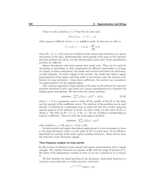
334 6 Approximation and fitting
Thus we seek a function f ∈ F that fits the data well,
f(u i ) ≈ y i , i = 1, . . . , m,
with a sparse coefficient vector x, i.e., card(x) small. In this case we refer to
f = x 1 f 1 + · · · + x n f n = ∑ x i f i ,
i∈B
where B = {i | x i ≠ 0} is the set of indices of the chosen basis elements, as a sparse
description of the data. Mathematically, basis pursuit is the same as the regressor
selection problem (see §6.4), but the interpretation (and scale) of the optimization
problem are different.
Sparse descriptions and basis pursuit have many uses. They can be used for
de-noising or smoothing, or data compression for efficient transmission or storage
of a signal. In data compression, the sender and receiver both know the dictionary,
or basis elements. To send a signal to the receiver, the sender first finds a sparse
representation of the signal, and then sends to the receiver only the nonzero coefficients
(to some precision). Using these coefficients, the receiver can reconstruct
(an approximation of) the original signal.
One common approach to basis pursuit is the same as the method for regressor
selection described in §6.4, and based on l 1 -norm regularization as a heuristic for
finding sparse descriptions. We first solve the convex problem
minimize
∑ m
i=1 (f(u i) − y i )) 2 + γ‖x‖ 1 , (6.18)
where γ > 0 is a parameter used to trade off the quality of the fit to the data,
and the sparsity of the coefficient vector. The solution of this problem can be used
directly, or followed by a refinement step, in which the best fit is found, using the
sparsity pattern of the solution of (6.18). In other words, we first solve (6.18), to
obtain ˆx. We then set B = {i | ˆx i ≠ 0}, i.e., the set of indices corresponding to
nonzero coefficients. Then we solve the least-squares problem
minimize
∑ m
i=1 (f(u i) − y i )) 2
with variables x i , i ∈ B, and x i = 0 for i ∉ B.
In basis pursuit and sparse description applications it is not uncommon to have
a very large dictionary, with n on the order of 10 4 or much more. To be effective,
algorithms for solving (6.18) must exploit problem structure, which derives from
the structure of the dictionary signals.
Time-frequency analysis via basis pursuit
In this section we illustrate basis pursuit and sparse representation with a simple
example. We consider functions (or signals) on R, with the range of interest [0, 1].
We think of the independent variable as time, so we use t (instead of u) to denote
it.
We first describe the basis functions in the dictionary. Each basis function is a
Gaussian sinusoidal pulse, or Gabor function, with form
e −(t−τ)2 /σ 2 cos(ωt + φ),