A 2D Finite Volume Non-hydrostatic Atmospheric Model ...

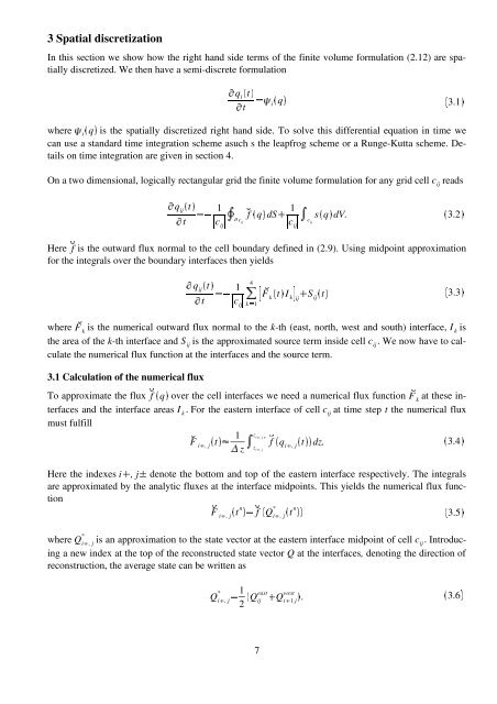
wrwHru€rwuwF k s t t I k| ij x S ij s t tw}ƒ}ƒ}3 Spatial discretizationIn this section we show how the right hand side terms of the finite volume formulation (2.12) are spatiallydiscretized. We then have a semi-discrete formulationq i t t su… ti s qt3.1~where g i h qi is the spatially discretized right hand side. To solve this differential equation in time wecan use a standard time integration scheme asuch s the leapfrog scheme or a Runge-Kutta scheme. Detailson time integration are given in section 4.On a two dimensional, logically rectangular grid the finite volume formulation for any grid cell c ijreadsq ijt t st1H D?Fcc ijijf s qt dS x1Hc ijHCc ij s s qt dV.s 3.2tHere f is the outward flux normal to the cell boundary defined in (2.9). Using midpoint approximationfor the integrals over the boundary interfaces then yieldsu*vq ijt t st14 {H H#yc ij 1 kz3.3„u vwhere jF kis the numerical outward flux normal to the k-th (east, north, west and south) interface, I kisthe area of the k-th interface and S ijis the approximated source term inside cell c ij. We now have to calculatethe numerical flux function at the interfaces and the source term.3.1 Calculation of the numerical fluxTo approximate l the flux kf over the cell interfaces we need a nnumerical flux function F qm kat these interfacesand the interface areas I k. For the eastern interface of cell c ijat time step t the numerical fluxmust fulfill1s F tS iq , jtzz f qC iq , j s t t.t dz. si , j‚z i , jw3.4~Here the o indexes i p , j denote the bottom and top of the eastern interface respectively. The integralsare approximated by the analytic fluxes at the interface midpoints. This yields the numerical flux functionF iq s , jt n *s f Q iq , s jt n t.tt3.5~*where Q iq , jis an approximation to the state vector at the eastern interface midpoint of cell c ij. Introducinga new index at the top of the reconstructed state vector Q at the interfaces, denoting the direction ofreconstruction, the average state can be written as*Q iq , j1Q east2 ijQ west iq 1 jt . x s3.6„7