A 2D Finite Volume Non-hydrostatic Atmospheric Model ...

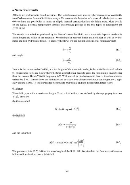
h c x dfe1‰ c x— adh c x dfe H exp – g c x— a dž‹6 Numerical resultsAll tests are performed in two dimensions. The initial atmospheric state is either isentropic or constantlystratified (constant Brunt-Väisälä frequency). To simulate the behavior of a thermal bubble (see section6.6) we have the possibility to insert an elliptic thermal perturbation into the initial state. More detailson the typical potential temperature, density and pressure profiles of the two types of atmosphere aregiven in [6].The steady state solutions produced by the flow of a stratified fluid over a mountain depends on the differentheight and width of the mountain. We distinguish between linear and nonlinear as well as hydrostaticand non-hydrostatic flows. To classify the flows we use the non-dimensional mountain widthand height6.1Œ‘h e h N u 0.6.2ŽHere a is the mountain half width, h is the height of the mountain and u 0is the initial horizontal velocity.Hydrostatic flows are flows where the time a parcel of air needs to cross the mountain is much biggerthan the inverse Brunt-Väisälä frequency 1/N. With use of (6.1) a hydrostatic flow is therefore characterizedby a 1. Linear flows are characterized by a low non-dimensional mountain height ‘h ’ 1 typicallyaround 0.001. To test our model we simulate hydrostatic and non-hydrostatic, linear flows.6.1 SetupThree hill types with a maximum height H and a half width a are defined by the topography functionh “ x” . They arethe Gaussian hilla q a N u 0‹h x c dfe H exp a – g c x—2˜d ,6.3Žthe Bell hillH26.4Œand the Schär hillx š› œ cos .22˜6.5ŽThe parameter • in (6.5) defines the wavelength of the Schär hill. We simulate the flow over a Gaussianhill as well as the flow over a Schär hill.23