A 2D Finite Volume Non-hydrostatic Atmospheric Model ...

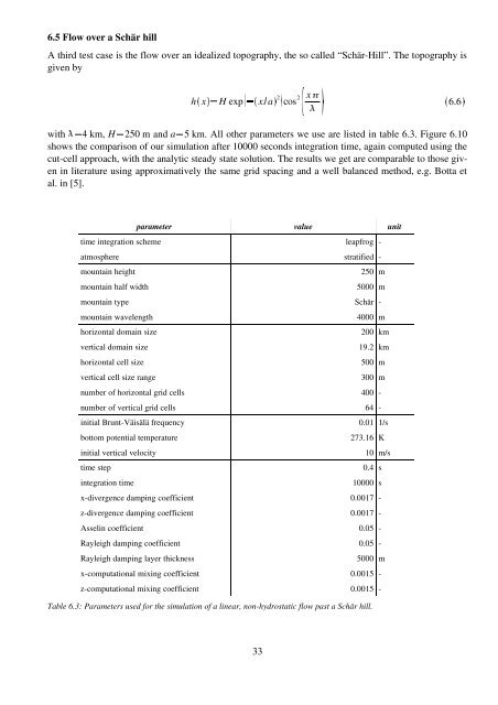
h c x dfe H exp – g c x— a dcos 2 x š›©œ‹6.5 Flow over a Schär hillA third test case is the flow over an idealized topography, the so called “Schär-Hill”. The topography isgiven by2˜6.6Œwith ¦¨§ 4 km, H e 250 m and a e 5 km. All other parameters we use are listed in table 6.3. Figure 6.10shows the comparison of our simulation after 10000 seconds integration time, again computed using thecut-cell approach, with the analytic steady state solution. The results we get are comparable to those givenin literature using approximatively the same grid spacing and a well balanced method, e.g. Botta etal. in [5].parameter value unittime integration schemeatmosphereleapfrogstratified--mountain heightmountain half widthmountain typemountain wavelength2505000Schär4000mm-mhorizontal domain sizevertical domain sizehorizontal cell sizevertical cell size rangenumber of horizontal grid cellsnumber of vertical grid cells20019.250030040064kmkmmm--initial Brunt-Väisälä frequencybottom potential temperatureinitial vertical velocity0.01273.16101/sKm/stime stepintegration timex-divergence damping coefficientz-divergence damping coefficientAsselin coefficientRayleigh damping coefficientRayleigh damping layer thicknessx-computational mixing coefficientz-computational mixing coefficient0.4100000.00170.00170.050.0550000.00150.0015ss----m--Table 6.3: Parameters used for the simulation of a linear, non-hydrostatic flow past a Schär hill.33