Probabilistic Seismic Demand Model for California Highway Bridges

Probabilistic Seismic Demand Model forCalifornia Highway BridgesKevin Mackie 1 AM ASCEBožidar Stojadinović 2 AM ASCEAbstractA performance-based seismic design method enables designers to evaluate a graduated suite ofperformance levels for a structure in a given hazard environment. The Pacific Earthquake EngineeringCenter is developing a framework for performance-based seismic design. One componentof this framework is a probabilistic seismic demand model for a class of structures in an urbanregion with a well-defined seismic hazard exposure. A probabilistic seismic demand model relatesground motion Intensity Measures to structural Demand Measures. It is formulated by statisticallyanalyzing the results of a suite of non-linear time-history analyses of typical structures underexpected earthquakes in the urban region. An example of a probabilistic seismic demand modelfor typical highway bridges in California is presented. It was formulated using a portfolio of 80recorded ground motions and a portfolio of 108 bridges generated by varying bridge design parameters.The sensitivity of the demand models to variation of bridge design parameters is alsodiscussed. Trends derived from this sensitivity study provide designers with a unique tool to assessthe effect of seismicity and design parameters on bridge performance.1 Graduate Student, University of California, Berkeley, Department of Civil & Env. Engineering2 Assistant Professor, University of California, Berkeley, Department of Civil & Env. Engineering, 721 Davis Hall#1710, Berkeley, CA 94720-1710, e-mail: boza@ce.berkeley.edu1

Keywordsperformance-based design, seismic hazard intensity measures, structural demand measures, probabilisticseismic design model, reinforced concrete bridges2

INTRODUCTIONPerformance-based design provides a means for structures to be designed to meet an array ofgraduated performance objectives in a specific hazard environment. Dealing with multiple performanceobjectives, each comprising a performance level at a seismic hazard level, requires a designframework significantly more complex than traditional seismic design frameworks. Recent implementationsof performance-based design frameworks, such as FEMA-273 [FEMA-273 96] andVision 2000 [SEAOC 95], account for location-specific seismic hazards in a probabilistic manner,where the graduated arrays of performance levels are based on deterministic estimates of structuralcapacities. A consistent probability-based approach, where uncertainties in the demand and capacitysides are considered simultaneously, has only been fully implemented recently in the SACSteel Project [FEMA-350 00] to design steel moment frame buildings.The Pacific Earthquake Engineering Research Center (PEER) is developing a consistent probabilitybasedframework for seismic performance-based design and evaluation. This framework draws onresults from the SAC Steel Project, but is substantially more general. Performance objectivesare defined in terms of socio-economic Decision Variables (DV) and annual probabilities that suchvariables will exceed specified limit values in a seismic hazard environment of the urban region andsite under consideration. However, a general probabilistic model directly relating Decision Variablesto seismic hazard Intensity Measures (IM) is too complex. Instead, the PEER performancebaseddesign framework utilizes the Joint Probability Theorem to de-aggregate various sources ofrandomness and uncertainty. Thus, the mean annual frequency of a DV exceeding limit value z is[Cornell 00]:ν DV ´zµ yxG DV DM´zyµ dG DMIM´yxµ dλ IM´xµ (1)The kernel of the double integral in Equation 1 comprises three probabilistic models:G DV DM´zyµ is a capacity model, predicting the probability of exceeding the value of a DecisionVariable z, given a value of a Demand Measure (DM) y;G DMIM´yxµ is a demand model, predicting the probability of exceeding value of a DemandMeasure y, given a value of a seismic hazard Intensity Measure (IM) x;dλ IM´xµ is a seismic hazard model, predicting the probability of exceeding the value of a seismic3

hazard Intensity Measure (IM) x in a given seismic hazard environment.Such de-aggregation is possible only if the three models involved are mutually independent, and ifthe capacity and demand models are independent of the seismic hazard environment. Furthermore,the intermediate variables IM, DM and DV should be chosen such that probability conditioningis not carried over from one model to the next. Finally, the models should be efficient, meaningthat the dispersion between the model and the data is small and constant over the entire rangeof model variables. Design of a good de-aggregated performance-based design framework is noteasy [Cornell 00]. However, such a de-aggregated approach is to performance-based design whatobject-oriented approach is to programming: it enables de-coupling of a large problem into independentunits. Such units can be designed separately and used interchangeably, making it easier todevelop a general performance-based framework for seismic design and evaluation.The hazard and performance de-aggregation process described above is depicted in Figure 1for the case of a highway overpass bridge. First, seismic hazards, evaluated using a regionalhazard model, are expressed using Intensity Measures. A demand model, built for this class ofbridges, is then used to correlate hazard Intensity Measures to structural Demand Measures for thisbridge. Next, a capacity model is used to relate structural Demand Measures to Decision Variables.Decision Variables describe the performance of a typical overpass bridge after an earthquake interms of its function in a traffic network in an urban region such as the San Francisco Bay Area.The results of a performance-based evaluation of an overpass bridge in the San Francisco Bay Areaare mean annual probabilities of exceeding set values of a chosen suite of Decision Variables.A probabilistic seismic demand model (PSDM hereafter) for typical California highway bridgesis presented in this paper. The fundamentals of developing a PSDM, such as the choice of groundmotions and their Intensity Measures, and the choice of bridge design parameters and structuralDemand Measures, are presented first. Sample PSDMs for a two-span single-bent highway overpassare derived and explored next. A discussion of how to formulate highway overpass PSDMsand how to incorporate them into PEER’s performance-based seismic design framework concludesthis paper.4

PROBABILISTIC SEISMIC DEMAND MODELA PSDM is a result of probabilistic seismic demand analysis. Probabilistic seismic demand analysis(PSDA), as defined in [Shome 98], is the coupling of probabilistic seismic hazard analysis(PSHA) and nonlinear structural analysis. PSDA is done to estimate the probabilities of exceedingdiscrete levels of structural demand measures in a postulated seismic hazard environment, i.e. toformulate a structural demand hazard curve [Luco 01].Nowadays, probabilistic seismic evaluation is routinely done as a part of performance-baseddesign of important and expensive structures such as the new East Bay Bridge across the San FranciscoBay. In such projects, a complex non-linear model of the structure is typically subjectedto a large number of real and artificial ground motions to estimate the required probabilities ofexceeding predetermined values of a set of project-specific Decision Variables. Such computationallyintensive approaches are applicable to unique structures only, and cannot be used in routineperformance-based design.A de-aggregated performance-based design framework (Equation 1) is a practical alternative.One step in this framework is a PSDA used to formulate a PSDM that applies to an entire urbanregion, rather than to a unique location; applies to an array of possible Decision Variables, ratherthan a single one; and applies to a class of structures, rather than to a unique structure. SuchPSDMs are quite general. The procedure used to formulate them has four aspects: choice ofground motions, definition of the class of structures, formulation of a non-linear analysis model,and choice of Intensity Measure and Demand Measure pairs to describe the model. Formulation ofPSDMs for typical California two-span single-column-bent highway overpass bridges will be usedto illustrate such PSDA procedure.Ground Motions for PSDACustomary probabilistic seismic hazard analysis yields hazard curves that relate measures of groundmotion intensity, such as peak ground acceleration, to earthquake (moment) magnitude (M w ) andepicentral distance (R) for an urban region. Such hazard curves, also called attenuation curves,are usually conditioned on local soil type. They are computed using an elastic single-degreeof-freedomsystem model to compute the required spectral quantities for a suite of measured or5

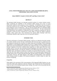
artificially generated earthquakes typical of the urban region under study.PSDA is not based on seismic hazard curves. Instead, a ground motion bin approach proposedby Shome and Cornell [Shome 98, Shome 99] is used. In this approach, a suite of ground motionstypical for the region under study is chosen from a database of recorded ground motions.Using magnitude and epicentral distance data, these ground motions are divided into bins. Separatingbins by magnitude and epicentral distance makes this strategy comparable to conventionalPSHA. One advantage of using bins is the ability to abstract individual earthquakes and considerthe effect of generalized earthquake characteristics, such as frequency domain content, dominantperiod, or duration, on structural demand. For example, bins differentiate between near- and farfieldearthquake types, rather than between individual near- and far-field records. Ground motionintensity can also be abstracted by scaling the earthquakes in a bin to the same level of intensity,such as spectral acceleration at the fundamental period of a structure. More importantly, the binapproach provides a way to limit the number of ground motions in the suite. Shome and Cornell[Shome 98] show that, assuming a log-normal probability distribution of structural DemandMeasures, the number of ground motions sufficient to yield response quantity statistics that havea required level of confidence is proportional to the square of a measure of dispersion of DemandMeasure data. They also show that proper scaling of bin intensities can reduce dispersion, and thussubstantially reduce the number of ground motions required for confident analysis. Finally, theyshow [Shome 99] that the bin approach by itself does not introduce bias into the relation betweenstructural Demand Measures and ground motion Intensity Measures.To date, there are no specific guidelines for choosing the ground motions for PSDA. To conductthe sample PSDA presented in this paper, a portfolio of 80 ground motions recorded in Californiawas assembled from the PEER Strong Motion Database available at [PEER Strong Motion Catalog ].This portfolio is characteristic of non-near-field ground motions recorded in California. It is similarto the portfolio used in a companion PEER project on buildings [Medina 00, Gupta 00], the differencesstemming from a requirement that all ground motions have all three orthogonal componentsrecorded in the database. All ground motions were recorded on NEHRP soil type D sites.This ground motion portfolio was divided into bins defined by moment magnitude M w andepicentral distance R, as shown in Figure 2. The delineation between small (SM) and large (LM)magnitude bins was at M w 65. Ground motions with epicentral distance R between 15 and 306

km were grouped into a small distance (SR) bin, while ground motions with R 30 km were inthe large distance (LR) bin. Ground motions with epicentral distance R smaller than 15 km wereintentionally omitted to eliminate the near-field effects from this PSDA study. The portfolio waschosen so that each bin contains 20 motions, distributed as uniformly as possible within each bin(Figure 2).Class of Structures for PSDAThe second component of a PSDA is the definition of a class of structures to be analyzed. A class ofstructures is defined by structural topology, typical structural components, and methods of design.Sample structures are instantiations of a class defined by specific geometry and design parameters.The goal of PSDA is to produce a PSDM that enables design parameter sensitivity investigations.The PSDA presented in this paper is conducted for a class of typical new California highwayoverpass bridges. Such bridges are constructed using reinforced concrete and designed accordingto Caltrans’ Bridge Design Specification and Seismic Design Criteria [Caltrans 99] which incorporaterecommendations from ATC-32 [Council 96]. Longitudinal structural configurations forbridges in this class are shown in Figure 3. They are: single-span, two-span, and three-span overpasses(including abutments) and stand-alone components of multi-span viaducts divided at expansionjoints. In the transverse direction, typical California overpasses have single, two-columnor multi-column bents (Figure 3). At abutments and expansion joints these bridges have varyingdegrees of restraint (shear keys and/or rubber bearing pads, for example). Common to all bridgesis a Type I integral pile shaft foundation extending into a column with a uniform cross-section, anda continuous superstructure, as designed by Caltrans [Yashinsky 00]. In this study it was assumedthat new bridge columns develop plastic hinges in flexure rather than failing in shear, consistentwith the displacement-based capacity design approach used by Caltrans.A two-span single-column bent highway overpass bridge class was chosen to demonstratePSDA in this paper (Figure 4). While actual bridge designs would be governed by Caltrans criteria,members of this bridge class were generated by varying ten bridge design parameters. They are:degree of skew, span length, span to column height ratio, steel and concrete nominal strengths,amount of longitudinal and transverse column reinforcement, ratio of column diameter to super-7

structure depth, soil properties at pile shafts, and bridge weight. These parameters are defined inFigure 4 and listed in Table 1 together with ranges of their variation used in this study.A base bridge configuration defined by zero angle of skew, two equal 18.2 m (60 ft) spans, a7.6 m (30 ft) high single-column bent, with a 1.6 m (5.25 ft) diameter circular column that has 2%longitudinal and 0.7% transverse reinforcement, and a Type I pile shaft foundation on a NEHRPclass D soil site. A suite of 108 different two-span overpass bridges was generated by varyingdesign parameters from the base configuration, one at a time. Such parameter variation was doneto cover the entire parameter space, even though it may generate a few uncommon bridge designs.Nonlinear Analysis for PSDANonlinear analysis is the third component of PSDA. The importance of choosing a nonlinear analysistool and understanding its limitations cannot be underestimated. This tool should enable sufficientlyaccurate modeling of the class of structures under investigation, perform stable nonlineartime-history analysis of the structure, and enable easy extraction and post-process various structuralresponse quantities after an analysis. More importantly, this analysis tool must be calibratedto give a level of confidence in the response quantities it produces.Nonlinear analysis of the sample PSDA presented in this paper was done using PEER’s OpenSeesplatform [McKenna 00, OpenSees ]. A nonlinear model for the base bridge configuration wasdeveloped first. The columns and pile shafts were modeled using a three-dimensional flexibilitybasednonlinear beam-column element with fiber cross sections. This element provides a nonlinearmodel for flexure and axial load effects, while effects of shear and torsion are modeled linearly,using initial uncracked stiffness. The circular column cross-sections have perimeter longitudinalbars and spiral confinement. A simple elastic-plastic material with a post-yield (hardening) stiffnessequal to 1.5% of pre-yield stiffness was used to model all reinforcement steel. Concrete confinedby the spirals was modeled using a Kent-Scott-Park stress-strain relation, with the maximumconfined concrete strength determined using Mander’s confinement model [Kent 71, Mander 88].Soil-structure interaction in pile shaft foundations was modeled using bi-linear springs at varyingdepths over the pile shaft length, as in [Fenves 98]. The properties of these p-y springs weredetermined using soil parameters and recommendations from API [Institute 93]. P ∆ effects were8

included in the analysis to capture the effect of tall columns and relatively heavy bridge decks. Thebridge deck was designed as a typical Caltrans box section for a three-lane wide roadway. Duringthe nonlinear analyses, the deck was assumed to remain elastic. Thus, it was modeled as a linearelastic beam, but with a cracked section stiffness.The abutments were modeled using nonlinear elastic-perfectly plastic spring-gap elements,which directly account for gap opening and closing. The longitudinal direction resistance ofthe abutment was derived from the stiffness of elastomeric bearing pads on seat-type abutments[Priestley 96]. The abutment stiffness model ignored the embankment and soil inertial effects.Instead, a passive earth pressure of the backwall, set at 370 KPa (7.7 ksf) according to the Caltransprocedure [Goel 97] which includes an empirical pile resistance estimate of 0.7 kN/m/pile(40kips/in/pile) [Maroney 94a], was used. The initial seat gap was assumed to be 15.2 cm (6in). Therefore, the longitudinal participation of the abutment will occur only under large bridgedeformations. The abutment model in the transverse direction has a similar stiffness as in the longitudinaldirection, provided by the shear keys, wing-walls and piles, but is activated immediately(there is a zero-length gap).Initial analyses showed that the response of short-span bridges is dominated by the dynamicresponse of the approach embankment and abutment. In order to make the bridge model morerealistic, spring properties derived above were “softened” by a factor of 2. Such softening alsoaddresses the discrepancy between the Caltrans-recommended stiffness and the tri-linear abutmentstiffness envelope observed in large scale abutment tests [Maroney 94b]. More advanced bridgemodels should incorporate more complex abutment models, including soil mass inertia and soilpileinteraction and embankment soils, such as the soil slice model [Wissawapaisal 00].Nonlinear models for each one of the 108 bridges in this PSDA were made by changing thebridge design parameters in a computer script that generated individual OpenSees input files.Modal analyses were performed first, using bridge models with simple supports at abutments toexclude their effect to compute bridge fundamental transverse and longitudinal periods as controlledby the column only. Nonlinear time-history analyses were conducted by running a suite of80 ground motions, unscaled and divided into four bins as discussed above, through each one ofthe 108 bridge models. A database of bridge response quantities was generated by post-processingthe results of the time-history analyses.9

Intensity Measures and Demand Measures for PSDAA PSDM relates ground motion Intensity Measures to structure-class-specific Demand Measures.Thus, the choice of IM–DM pairs in the demand model is critical for a successful PSDA. Anoptimal PSDM should be practical, sufficient, effective and efficient, as described below.An IM–DM pair in a demand model is practical if it makes engineering sense and if it canbe easily derived from available ground motion measurements (for IMs) and nonlinear analysisresponse quantities (for DMs). Good correlations between computer model results and existingexperimental data lend further credibility to the model.From the standpoint of the performance-based design framework (Equation 1), it is importantthat both Intensity and Demand Measures are not statistically dependent on ground motion characteristics,such as moment magnitude and epicentral distance. Otherwise, de-aggregation can not beachieved. Demand models with such conditional statistical independence are said to be sufficient.Effectiveness of a demand model is a measure of how readily it yields itself to use in a deaggregatedperformance-based design framework. Assuming that ground motion Intensity Measureshave a log-normal distribution [Shome 98], an effective demand model should have a correspondingexponential form:DM a ´IMµ b (2)or, equivalentlylog´DMµA·B log´IMµ (3)making a log-log plot of the IM–DM relation specified by this demand model a straight line.More importantly, such a log-log linear (or piece-wise linear) demand model makes it possible toevaluate the integrals in the de-aggregated performance-based design framework (Equation 1) inclosed form and to cast the entire framework in an LRFD format. This was accomplished for steelmoment frames in the SAC Joint Venture Steel Project [FEMA-350 00, Cornell 01] and proved tobe crucial for wide adoption of probabilistic performance-based design in practice.A PSDM is derived by correlating Intensity Measures for ground motions in the ground motionportfolio and Demand Measures for the structure computed using nonlinear time-history analysis.A linear regression analysis of the logarithms of the IM–DM data gives coefficients A and B inEquations 2 and 3, and produces a line through the cloud of IM–DM data in a log-log plot as10

shown in Figure 5. Dispersion δ of the IM–DM data with respect to the regression fit, defined asthe standard deviation of the logarithm of regression residuals for Demand Measure [Shome 98](Figure 5), measures the variability of DM given IM. An efficient demand model has small dispersion,thus requiring a smaller number of different non-linear time-history analyses to computecoefficients A and B with the same confidence.Selecting an Intensity and Demand Measure pair for a practical, sufficient, effective and efficientPSDM is not easy. The traditional relation between Peak Ground Acceleration and structuralresponse is practical, but is neither efficient nor effective. A number of Intensity Measure–DemandMeasure pairs presented in the literature in recent years have been aimed at performance-based designof buildings. Thus, a principal milestone in the development of a PSDM for highway overpassbridges is the search for an optimal Intensity and Demand Measure pair for this class of structures.The search for an optimal IM–DM pair is best done with the aid of computers. This enablesconsideration of a large number of Intensity and Demand measure combinations. The groundmotion Intensity Measures used in this study are shown in Table 2. These measures range fromconventional spectral quantities, across duration and energy-related quantities, to characteristicsof the ground motion frequency spectra. Each Intensity Measure is ground motion specific, yetindependent of the bridge model. Intensity Measures for the selected ground motion records werecomputed in advance and stored in a database.Bridge Demand Measures were chosen from a recently developed PEER database of experimentalresults for concrete bridge components [Hose 00, PEER Capacity Catalog ]. These DemandMeasures, listed in Table 3, span from global ones, such as bridge drift ratio, to intermediateones, such as cross-section curvature, to local ones, such as steel and concrete strain. The OpenSeesbridge model is programmed to output a record of Demand Measures after each time-history analysis.This record is also stored in a database. After completing 80 response-history analyses for eachof the 108 bridges, the resulting database can be searched enabling arbitrary paring of Intensity andDemand Measures and pair-to-pair comparison.11

SAMPLE PSDADevelopment of a PSDM is illustrated in this sample PSDA. The class of structures under considerationis a two-span single-bent straight highway overpass bridge. The base bridge has no skewat the abutments. Each span is 18.2 m (60 ft) long. The bent comprises a single 7.6 m (30 ft) tallcolumn, measured from the soil surface. This column has a 1.6 m (5.25 ft) diameter circular crosssection with 2% longitudinal and 0.7% transverse reinforcement. The column foundation is anintegral Type I pile shaft. This base bridge is on a NEHRP class D soil site. The ground motionsused in this PSDA were the 80 ground motions classified into four bins shown in Figure 2. Thesemotions were not scaled in intensity or modified in any way. They were arbitrarily oriented so thatthe fault-normal component was applied in the longitudinal direction of the bridge.The scope of parameter variation presented herein was intentionally reduced to fit the format ofthis paper. Only two ground motion Intensity Measures were considered. They are S d1 ln and S d1 tr,elastic 5%-damping Spectral Displacements at the fundamental longitudinal and transverse periodsof the bridge, respectively (Table 2). Only six Demand Measures were considered. They are:bridge displacement ductility, bridge column curvature ductility, and bridge residual displacementin both transverse and longitudinal directions each (Table 3). Lastly, only 10 different bridgesare considered by varying three design parameters, namely span to column height, longitudinalcolumn reinforcement, and ratio of column diameter to superstructure depth with respect to thebase bridge configuration (Table 4). Only one parameter was varied from the base configuration ata time, while the other two were kept constant.Modal analysis of the 10 bridge models yields the periods of the first two elastic vibrationmodes listed in Table 4. The first two mode shapes were practically identical for all 10 consideredbridges. The first mode shape is dominated by longitudinal deck motion accompanied by smalldeck rotations near the abutments. The second mode shape is dominated by simple transversemotion of the deck. The longitudinal and transverse periods for each of the bridges were used tocompute the Intensity Measures S d1 ln and S d1 tr for the 80 ground motions involved. Followingmodal analyses, 800 nonlinear time-history analyses were done using the OpenSees finite elementmodel. The Demand Measures from these analyses were computed and stored in the database forlongitudinal and the transverse bridge directions independently.12

Resulting PSDMsDifferent PSDMs are shown in Figures 6 through 18. In each of these figures, the data is plotted inlog-log scale, with the Demand Measure on the abscissa and the Intensity Measure on the ordinate.This is a standard method for plotting any IM–DM relationship (stemming from a push-over curveaxis designation) even though the Demand Measure is regarded as the dependent variable. Aregression analysis of the data yields coefficients A and B of Equation 3 listed in Table 5. Alsolisted are values of dispersion δ for each regression analysis to characterize the efficiency of theprobabilistic seismic demand model. In this example, only a single linear fit to the data was made.Smaller dispersion can be achieved using a bi- or tri-linear fit not performed in this example.Model ComparisonThis PSDM pairs Spectral Displacement at the fundamental period of the bridge as the IntensityMeasure and bridge column Curvature Ductility as the Demand Measure. PSDMs for longitudinaland transverse directions of the base bridge are shown in Figures 6 and 7, respectively. Dataregressions were done separately for each of the four ground motion bins shown in Figure 2. Asexpected, more intense ground motions induce larger column curvature demands (the large magnitude,small distance bin). Single-line fitting (Equation 3) produces a good PSDM, with dispersionsδ ranging between 0.20 and 0.43. Thus, the Spectral Displacement–Column Curvature demandmodel is an effective and efficient model, but may not be practical from a design standpoint.A PSDM comprising Spectral Displacement and column Displacement Ductility is shown inFigures 8 and 9, respectively. The Demand Measure in this model (column displacement ductility)was chosen because it is more practical for design than curvature ductility. This model wasintended to capture the effect of inelastic shear deformation on the performance of the bridge. Albeit,the beam-column element used in this implementation of the OpenSees includes only elasticshear deformation, enabling a direct relation between column curvature and column displacement.Thus, the quality of this PSDM is similar to the PSDM examined above. This example illustratesthe need for careful consideration of the analysis tools used for PSDA. The resulting PSDMs willonly be as good as the analytical models used to compute them.A third PSDM pairs Spectral Displacement with a column Residual Displacement Index (RDI13

in Table 3). RDI measures the amount of residual inelastic deformation of the structure after anearthquake. The model is shown in Figures 10 and 11. Data in this model has a huge scatter, notonly between bins but also within each bin. Values of dispersion of each regression line are onthe order of 0.80, two to three times larger than for the two PSDMs discussed above. Such largescatter makes this model ineffective and inefficient, even though it has a well-defined meaning forbridge design. This example shows how to evaluate the quality of PSDMs.Design Parameter SensitivityA good PSDM my be used as a design tool for discovering how changes in different design parametersaffect the performance of a bridge. The Spectral Displacement–Column Curvature DemandPSDM will be used in the following.The effects of variation of the bridge span-to-column height ratio (span fixed, height determinedby ratio) are shown in Figures 12 and 13, all ground motions included. Evidently, as the span-tocolumnheight ratio is increased (i.e. the bridge is becoming more squat, and more stiff comparedto the base configuration, going from left to right across the graphs) column curvature ductilityDemand Measure increases for constant values of Spectral Displacement Intensity Measure. Theslope of the linear regression fit is steeper for smaller the span-to-height ratios, meaning that stifferbridges have a higher rate of increase of curvature demand with the increase of bridge span-tocolumnheight ration. However, the fundamental period of a stiffer bridge will be shorter, leadingto smaller values of Spectral Displacement Intensity Measure. Therefore, given the range of bridgeperiods considered, increasing bridge stiffness by reducing the span-to-column height ratio resultsin either no net gain, or even a loss of performance. To a designer this would suggest alternatemethods are required for reducing column ductility demand.The effects of varying the column diameter are examined using PSDMs in Figures 14 and 15,using the column diameter-to-superstructure depth ratio as the design parameter. In contrast to thespan-to-column height parameter, increasing bridge stiffness by increasing the column diameterhas the direct effect of lowering curvature ductility demand (stiffness increases from right to leftin the graphs). Dispersions δ are on the order of 0.25 and insensitive to variation of the designparameter. Therefore, changing column diameter is a better way to decrease column curvaturedemand.14

Variation of the amount of longitudinal reinforcing steel in the column is examined using PS-DMs shown in Figures 16 and 17. Stiffening and strengthening the column by providing more steelhas a similar effect as increasing column diameter. As expected, more reinforcement reduces ductilitydemand for more intense motions when the response of the column becomes inelastic, whileadding reinforcement has a negligible effect for low-intensity ground motions when the column iselastic. In contrast, the effect of changing column diameter was evident at all ground motion intensitylevels. The PSDMs show that performance improvement rate saturates as more reinforcementis added. The reduction in curvature demand obtained by increasing the amount of longitudinalreinforcement from 1% to 2% is significantly larger than the reduction obtained by increasing theamount of steel from 3% to 4%. Also of note is the magnitude of dispersion δ. It depends on theamount of reinforcement, being the largest for ρ = 1%. This suggests that more heavily reinforcedcolumns have more uniform behavior across the range of ground motions considered in this study.Finally, effect of abutment modeling is examined in Figure 18, for transverse bridge directiononly. Two bridge models are used to generate PSDMs in this figure. One model utilizes springswhose stiffness was computed using abutment stiffness data. This model was used for other PS-DMs in this example. The other model has roller supports instead of springs, assuming abutmentsdo not participate in bridge response. As expected, abutment participation adds strength to thebridge and reduces demand at any given ground motion intensity level. Unfortunately, these PS-DMs can not be used to determine which abutment model is more realistic: more field test data isneeded to calibrate abutment models.CONCLUSIONProbabilistic seismic demand models for typical California highway overpass bridges were presentedin this paper. They were developed using probabilistic seismic demand analysis for a classof real structures. Using a class of realistic structures, rather than a somewhat artificial singledegree-of-freedomsystem model, is a fundamental extension of PSDA. While preparing for PSDAan analyst should consider the following issues:1. Choice of ground motion Intensity Measures and structural Demand Measures should bemade to produce a practical, sufficient, effective and efficient PSDM. Guidelines for making15

such choices are as yet scarce.2. Reducing the dispersion in PSDMs is a high-priority task, since it directly affects the numberof ground motions and time history analyses required to compute PSDM parameters.3. When choosing the ground motions for PSDA, care should be taken to avoid bias, yet toaccurately represent the seismicity of the region for which PSDMs are being developed.4. Understanding the capabilities and shortcomings of the tool used to model and analyze thestructure is essential for proper interpretation of PSDMs.5. A class of structures is represented by a base structure and a number of instantiations developedby varying a set of design parameters. Therefore, good design of the base structure andprudent choice of design parameters are essential for successful development of PSDMs.6. The computational effort required to develop PSDMs for a class of structures and the complexityof the database required to track the results of a large number of analyses should notbe underestimated. Task scheduling, database and visualization tools should be designed andimplemented with care.Probabilistic seismic demand models for a class of structures provide information about theprobability of exceeding critical levels of chosen structural demand measures in a given seismichazard environment. Standing alone, PSDMs are, essentially, structural demand hazard curves.Given that they are developed for a class of structures, they provide information on how variationsof structural design parameters change the expected demand on the structure. Such sensitivity datacan be used to efficiently design structures for performance. The stand-alone value of PSDMs isfurther increased when they are used in a performance-based seismic design framework, such asthe one developed by PEER. In such design frameworks, PSDMs are coupled with ground motionintensity models on one side and structural element fragility models on the other side to yieldprobabilities of exceeding structural performance levels for a structure in a given seismic hazardenvironment.Probabilistic seismic demand models presented in this paper can be improved in several differentways. One aspect is the improvement of bridge models, such as improved modeling of column16

shear response and better abutment models. Another aspect is the investigation of how sensitivethe models are to the choice of ground motions (near-field vs. far-field) and local soil conditions. Athird way of improving PSDMs is by focusing on measures that evaluate the ability of the bridge tofulfill its function after an earthquake. Three sample function-related overpass Demand Measuresare: 1) enforcement of a 30 km/h speed limit and a 10-metric-ton axis weight limit for a period of 6weeks; 2) closure of one-half of bridge lanes for a period shorter than 2 weeks; and 3) maintenanceof bridge traffic at current levels after an after-shock that produces no more than 10 cm spectraldisplacement at first transverse period of the bridge. Such function-related Demand Measures enablea more direct evaluation of a bridge within a transportation network in an urban area, andbetter modeling of performance of such networks after earthquakes. Work on these improvementsis ongoing.ACKNOWLEDGMENTThis work is supported by the Earthquake Engineering Research Centers Program of the NationalScience Foundation under Award Number EEC-9701568 as PEER Project #312-2000 “SeismicDemands for Performance-Based Seismic Design of Bridges”. The authors gratefully acknowledgethis support. The opinions presented in this paper are solely those of the authors and do notnecessarily represent the views of the sponsors. The authors are also grateful to Professor C. AllinCornell and a group of his graduate students at Stanford University for enlightening discussionsabout PSDMs.17

APPENDIX: REFERENCES[Caltrans 99] Caltrans,. Seismic Design Criteria. California Department ofTransportation, 1.1 edition, July 1999.[Cornell 00]Cornell, C. A. and Krawinkler, H. . “Progress and challengesin seismic performance assessment.” PEER Center News, 3(2),Spring 2000.[Cornell 01] Cornell, C. A. , Jalayer, F. , Hamburger, R. O. , and Foutch, D. A.. “The probabilistic basis for the 2000 SAC/FEMA steel momentframe guidelines.” ASCE, Journal of Structural Engineering,2001. In press.[Council 96][FEMA-273 96][FEMA-350 00][Fenves 98][Goel 97]Council, A. T. . “Improved seismic design criteria for californiabridges.”. Report ATC-32, 1996. Palo Alto, CA.NEHRP guidelines for the seismic rehabilitation of buildings.Federal Emergency Management Agency (FEMA), WashingtonD.C., fema-273 edition, 1996.Recommended Seismic Design Criteria for New Steel Moment-Frame Buildings. Federal Emergency Management Agency(FEMA), Washington D.C., fema-350 edition, July 2000.Fenves, G. L. and Ellery, M. . “Behavior and failure analysis ofa multiple-frame highway bridge in the 1994 Northridge earthquake.”Technical Report 98/08, PEER, University of California,Berkeley, 1998.Goel, R. K. and Chopra, A. . “Evaluation of bridge abutmentcapacity and stiffness during earthquakes.” Earthquake Spectra,13(1):1–23, February 1997.18

[Gupta 00][Hose 00][Institute 93][Kent 71][Kramer 96][Luco 01][Mander 88][Maroney 94a]Gupta, A. and Krawinkler, H. . “Behavior of ductile of SRMFs atvarious hazard levels.” ASCE Journal of Structural Engineering,126(ST1):98–107, January 2000.Hose, Y. , Silva, P. , and Seible, F. . “Development of a performanceevaluation database for concrete bridge components andsystems under simulated seismic loads.” EERI Earthquake Spectra,16(2):413–442, April 2000.Institute, A. P. . “Recommended practice for planning, designing,and constructing fixed offshore platform: Load and resistancefactor design.”. Technical Report RP2A-LRFD, 1993. WashingtonD.C.Kent, D. C. and Park, R. . “Flexural members with confined concrete.”Journal of Structural Engineering, 97(ST7):1969–1990,July 1971.Kramer, S. L. . Geotechnical Earthquake Engineering. PrenticeHall, Upper Saddle River, NJ, 1996.Luco, N. , Cornell, C. A. , and Yeo, G. L. . “Annual limit-statefrequencies for partially-inspected earthquake-damaged buildings.”In 8th International Conference on Structural Safety andReliability, International Association for Structural Safety andReliability (IASSAR), Denmark, 2001. In press.Mander, J. B. , Priestley, M. J. N. , and Park, R. . “Theoreticalstress-strain model for confined concrete.” Journal of the StructuralEngineering, 114(ST8):1804–1826, August 1988.Maroney, B. , Kutter, B. , Romstad, K. , Chai, Y. H. , and Vanderbilt,E. . “Interpretation of large scale bridge abutment test19

esults.” In 3rd Annual Seismic Research Workshop, Caltrans,Sacramento, CA, 1994.[Maroney 94b][McKenna 00]Maroney, B. H. and Chair, Y. H. . “Seismic design and retrofittingof reinforced concrete bridges.” In 2nd International. Workshop,pages 255–276, Earthquake Commission of New Zealand,Queenstown, New Zealand, 1994.McKenna, F. and Fenves, G. L. . “An object-oriented software designfor parallel structural analysis.” In Advanced Technology inStructural Engineering, Proceedings, Structures Congress 2000,ASCE, Washington, D. C., 2000.[Medina 00] Medina, R. and Krawinkler, H. . “Seismic demands forperformance-based design.” Internal PEER Technical Report,November 2000.[OpenSees ][PEER Capacity Catalog ]http://www.opensees.org,. Web page.http://www.structures.ucsd.edu/PEER/CapacityCatalog/capacity catalog.html,. Web page.[PEER Strong Motion Catalog ] http://peer.berkeley.edu/smcat,. Web page.[Priestley 96]Priestley, M. J. N. , Seible, F. , and Calvi, G. M. . Seismic Designand Retrofit of Bridges. John Wiley and Sons, Inc., New York,NY, 1996.[SEAOC 95] SEAOC,. Vision 2000: A framework for performance baseddesign. Structural Engineers Association of California, Sacramento,CA, 1995.[Shome 98] Shome, N. , Cornell, C. A. , Bazzurro, P. , and Caraballo, J. E.. “Earthquakes, records, and nonlinear responses.” EERI EarthquakeSpectra, 14(3):467–500, June 1998.20

[Shome 99][Wissawapaisal 00][Yashinsky 00]Shome, N. and Cornell, C. A. . “Probabilistic seismic demandanalysis of nonlinear structures.” Reliability of Marine StructuresReport RMS–35, Department of Civil and EnvironmentalEngineering, Stanford University, Stanford, CA, 1999.Wissawapaisal, C. and Aschheim, M. . “Modeling the transverseresponse of short bridges subjected to earthquakes.” TechnicalReport 00-05, Mid-America Earthquake Center, University ofIllinois, Urbana-Champaign, IL, September 2000.Yashinsky, M. and Ostrom, T. . “Caltrans’ new seismic designcriteria for bridges.” EERI Earthquake Spectra, 16(1):285–307,February 2000.21

LIST OF FIGURE CAPTIONSFigure 1: PEER performance-based design frameworkFigure 2: Ground motion portfolio divided into binsFigure 3: Members of a highway overpass bridge class of structuresFigure 4: Design parameters for a two-span overpass bridgeFigure 5: Dispersion of IM–DM data with respect to a regression fit (Equation 2)Figure 6: PSDM pairing spectral displacement and column curvature ductility in longitudinalbridge directionFigure 7: PSDM pairing spectral displacement and column curvature ductility in transverse bridgedirectionFigure 8: PSDM pairing spectral displacement and column residual displacement index in longitudinalbridge directionFigure 9: PSDM pairing spectral displacement and column displacement ductility in transversebridge directionFigure 10: PSDM pairing spectral displacement and column residual displacement index in longitudinalbridge directionFigure 11: PSDM pairing spectral displacement and residual displacement index in transversebridge directionFigure 12: Sensitivity of the spectral displacement–column curvature ductility PSDM wrt. spanto-heightratio in longitudinal bridge directionFigure 13: Sensitivity of the spectral displacement–column curvature ductility PSDM wrt. spanto-heightratio in transverse bridge directionFigure 14: Sensitivity of the spectral displacement–column curvature ductility PSDM wrt. columndiameter in longitudinal bridge directionFigure 15: Sensitivity of the spectral displacement–column curvature ductility PSDM wrt. columndiameter in transverse bridge directionFigure 16: Sensitivity of the spectral displacement–column curvature ductility PSDM wrt. columnlongitudinal reinforcement ratio in longitudinal bridge directionFigure 17: Sensitivity of the spectral displacement–column curvature ductility PSDM wrt. column22

longitudinal reinforcement ratio in transverse bridge directionFigure 18: Sensitivity of the spectral displacement–column curvature ductility PSDM wrt. abutmentmodel in transverse bridge direction23

0 5 10 15 20 25 30 35HazardPerformance0.150.1acceleration [g]0.050-0.05-0.1time [sec]IntensityMeasuresDecisionVariablesDemandModelDemandMeasuresCapacityModelFigure 1: PEER performance-based design framework.24

Ground Motion BinsLMSRLMLR6.86.6Moment Magnitude M6.46.265.8SMSRSMLR0 10 20 30 40 50 60 70Distance R (km)Figure 2: Ground motion portfolio divided into bins.25

xxxxxxxxxxxxxxxxxxxxxxxxxxxxxxxxxxxxxxxxxxxxxxxxxxxxxxxxxxxxxxxxxxxxxxxxxxxxxxxxxxxxxxxxxxxxxxxxxxxxxxxxxxxxxxxxxxxxxxxxxxxxxxxxxxxxxxxxxxxxxxxxxxxxxxxxxxxxxxxxxxxxxxxxxxxxxxxxxxxxxxxxxxxxxxxxxxxxxxxxxxxxxxxxxxxxxxxxxxxxxxxxxxxxxxxxxxxxxxxxxxxxxxxxxxxxxxxxxxxxxxxxxxxxxxxxxxxxxxxxxxxxxxxxxxxxxxxxxxxxxxxxxxxxxxxxxxxxxxxxxxxxxxxxxxxxxxxxxxxxxxxxxxxxxxxxxxxxxxxxxxxxxxxxxxxxxxxxxxxxxxxxxxxxxxxxxxxxxxxxxxxxxxxxxxxxxxxxxxxxxxxxxxxxxxxxxxxxxxxxxxxxxxxxxxxxxxxxxxxxxxxxxxxxxxxxxxxxxxxxxxxxxxxxxxxxxxxxxxxxxxxxxxxxxxxxxxxxxxxxxxxxxxxxxxxxxxxxxxxxxxxxxxxxxxxxxxxxxxxxxxxxxxxxxxxxxxxxxxxxxxxxxxxxxxxxxxxxxxxxxxxxxxxxxxxxxxxxxxxxxxxxxxxxxxxxxxxxxxxxxxxxxxxxxxxxxxxxxxxxxxxxxxxxxxxxxxxxxxxxxxxxxxxxxxxxxxxxxxxxxxxxxxxxxxxxxxxxxxxxxxxxxxxxxxxxxxxxxxxxxxxxxxxxxxxxxxxxxxxxxxxxxxxxxxxxFigure 3: Members of a highway overpass bridge class of structures.26

xxxxxxxxxxxxxxx2LKabDcDsKabHAAxxxxxxxxxxxxxxxxxxxxxxxxxxxxxxxxxxxxxxxxxxxxxxxxxxxxxxxxxxxxxxxxxxxxxxxxxxxxxxxxxxxxxxxxxxxxxxxxxxxxxxxxxxxxxxxxxxxxxxxxxxxxxxxxxxxxxxxxxxxxxxxxxxxxxxxxxxxxxxxxxxxxxxxxxxxxxxxxxxxxxxxxxxxxxxxxxxxxxxxxxxxxxxxxxxxxxxxxxxxxxxxxxxxxxxxxxxxxxxxxxxxxxxxxxxxxxxxxxxxxxxxxxxxxxxxxxxxxxxxxxxxxxxxxxxxxxxxxxxxxxxxxxxxxxxxxxxxxxxxxxxxxxxxxxxxKsoilxxxxxxxxxxxxxxxxxxxxxA-AxxxxxxxxxFigure 4: Design parameters for a two-span overpass bridge.27

Intensity MeasureEquation (3)δδDemand MeasureFigure 5: Dispersion of IM–DM data with respect to a regression fit (Equation 2).28

10 1 Curvature Ductility LongitudinalSd T 1Longitudinal (cm)10 010 −1 10 0LMSRLMLRSMSRSMLRFigure 6: PSDM pairing spectral displacement and column curvature ductility in longitudinalbridge direction.29

Sd T 2Transverse (cm)10 110 0Curvature Ductility TransverseLMSRLMLRSMSRSMLR10 −1 10 0Figure 7: PSDM pairing spectral displacement and column curvature ductility in transverse bridgedirection.30

Sd T 1Longitudinal (cm)10 110 0Displacement Ductility LongitudinalLMSRLMLRSMSRSMLR10 −1 10 0Figure 8: PSDM pairing spectral displacement and column displacement ductility in longitudinalbridge direction.31

Sd T 2Transverse (cm)10 110 0Displacement Ductility TransverseLMSRLMLRSMSRSMLR10 −1 10 0Figure 9: PSDM pairing spectral displacement and column displacement ductility in transversebridge direction.32

Sd T 1Longitudinal (cm)10 110 0RDI LongitudinalLMSRLMLRSMSRSMLR10 −4 10 −3 10 −2 10 −1Figure 10: PSDM pairing spectral displacement and column residual displacement index in longitudinalbridge direction.33

Sd T 2Transverse (cm)10 110 0RDI TransverseLMSRLMLRSMSRSMLR10 −3 10 −2 10 −1Figure 11: PSDM pairing spectral displacement and column residual displacement index in transversebridge direction.34

10 1 Curvature Ductility LongitudinalSd T 1Longitudinal (cm)10 010 −1 10 0L/H=2.4L/H=2L/H=1.5L/H=1.2Figure 12: Sensitivity of the spectral displacement–column curvature ductility PSDM wrt. spanto-heightratio in longitudinal bridge direction.35

Sd T 2Transverse (cm)10 110 0Curvature Ductility TransverseL/H=2.4L/H=2L/H=1.5L/H=1.210 −1 10 0Figure 13: Sensitivity of the spectral displacement–column curvature ductility PSDM wrt. spanto-heightratio in transverse bridge direction.36

Sd T 1Longitudinal (cm)10 110 0Curvature Ductility LongitudinalDc/Ds=0.67Dc/Ds=0.75Dc/Ds=1Dc/Ds=1.310 −1 10 0 10 1Figure 14: Sensitivity of the spectral displacement–column curvature ductility PSDM wrt. columndiameter in longitudinal bridge direction.37

Sd T 2Transverse (cm)10 110 0Curvature Ductility TransverseDc/Ds=0.67Dc/Ds=0.75Dc/Ds=1Dc/Ds=1.310 −2 10 −1 10 0Figure 15: Sensitivity of the spectral displacement–column curvature ductility PSDM wrt. columndiameter in transverse bridge direction.38

Sd T 1Longitudinal (cm)10 110 0Curvature Ductility Longitudinalρ s,ln=0.01ρ s,ln=0.02ρ s,ln=0.03ρ s,ln=0.0410 −1 10 0 10 1Figure 16: Sensitivity of the spectral displacement–column curvature ductility PSDM wrt. columnlongitudinal reinforcement ratio in longitudinal bridge direction.39

Sd T 2Transverse (cm)10 110 0Curvature Ductility Transverseρ s,ln=0.01ρ s,ln=0.02ρ s,ln=0.03ρ s,ln=0.0410 −1 10 0 10 1Figure 17: Sensitivity of the spectral displacement–column curvature ductility PSDM wrt. columnlongitudinal reinforcement ratio in transverse bridge direction.40

Arias Intensity Transverse (cm/s)10 210 1Curvature Ductility TransverseNo abutmentAbutment10 −1 10 0Figure 18: Sensitivity of the spectral displacement–column curvature ductility PSDM wrt. abutmentmodel in transverse bridge direction.41

LIST OF TABLE CAPTIONSFigure 1: Parameter variation ranges for a two-span overpass bridgeFigure 2: Ground motion Intensity Measures considered in this study (source: [Kramer 96])Figure 3: Bridge Demand Measures considered in this studyFigure 4: Bridge first (longitudinal) and second (transverse) mode periodsFigure 5: Regression coefficients A and B (Equation 3) and dispersion δ for data in Figures 6through 1742

Table 1: Parameter variation ranges for a two-span overpass bridge.Description Parameter RangeDegree of skew α 0–π3 radSpan length L 18–55 m (60–180 ft)Span-to-column height ratio LH 1.2–2.4Column-to-superstructure dimension ratio D c D s 0.67-1.33Reinforcement nominal yield strength f y 470–655 MPa (68–95 ksi)Concrete nominal strength fc ¼ 20–55 MPa (3–8 ksi)Column longitudinal reinforcement ratio ρ sl 1–4%Column transverse reinforcement ratio ρ st 0.4–1.0%Soil stiffness based on NEHRP groups K soil A, B, C, DAdditional bridge dead load W da 10-100% self-weight43

Table 2: Ground motion Intensity Measures considered in this study (source: [Kramer 96]).Intensity MeasureDescription/equationArias Intensity I s π 2gÊ ∞0 ü 2 g´tµ dtVelocity Intensity I v Ê ∞0ü 2 g´tµ ˙u g´tµdtCumulative absolute velocityI A Ê ∞0 ü g´tµ dtCumulative absolute displacement I V Ê ∞0 ˙u g´tµ dtFrequency ratio 1Frequency ratio 2Strong motion durationFR 1 ˙u gmaxü gmaxFR 2 u gmax ˙u gmaxT d 002e 074M · 03RRMS accelerationCharacteristic intensityEffective peak accelerationEffective peak velocityEffective peak displacementa rms Õ 1TdÊ Td0 ü2 g´tµ dtI c a 15rms T 15dEPA 04 S aavg 0501EPV 04 S vavg 0501EPD 04 S davg 0501Spectral quantities S d S v ω S a ω 2Epicentral distanceMoment magnitudeRM44

Table 3: Bridge Demand Measures considered in this studyDemand MeasurePeak steel strainPeak concrete strainPeak column curvatureCurvature ductilityDisplacement ductilityDrift ratioResidual deformation indexEquationε smaxε cmaxφ m axµ φ φ max φ yµ ∆ u max u yγ u max HRDI u residual u yPlastic rotation θ p ´u max u y µHHysteretic energyHE À FduNormalized hysteretic energy NHE HE´F y u y µ45

Table 4: Bridge first (longitudinal) and second (transverse) mode periods.Bridge configuration T 1l [sec] T 1t [sec]1 Base bridge 0.56 0.352 LH 20 0.65 0.373 LH 15 0.81 0.384 LH 12 0.97 0.395 D c D s 067 0.64 0.366 D c D s 10 0.41 0.337 D c D s 13 0.33 0.308 ρ sl 001 0.59 0.359 ρ sl 003 0.54 0.3510 ρ sl 004 0.53 0.3546

Table 5: Regression coefficients A and B (Equation 3) and dispersion δ for data in Figures 6through 17.FigureABδLine 1 Line 2 Line 3 Line 46 a -2.28, 1.05, 0.43 -2.14, 0.73, 0.20 -2.33, 0.89, 0.22 -2.38, 0.93, 0.247 -2.34, 1.01, 0.42 -2.01, 0.53, 0.30 -2.31, 0.76, 0.30 -2.34, 0.76, 0.268 -2.17, 0.79, 0.20 -2.19, 0.72, 0.17 -2.36, 0.81, 0.16 -2.42, 0.85, 0.169 -2.00, 0.67, 0.26 -1.90, 0.46, 0.26 -2.21, 0.68, 0.24 -2.26, 0.63, 0.2310 -5.30, 0.92, 0.63 -5.06, 0.83, 0.81 -5.38, 0.63, 0.98 -4.95, 0.32, 0.9111 -5.84, 1.22, 0.77 -4.62, 0.53, 0.61 -4.92, 0.53, 0.73 -4.56, 0.56, 0.7712 b -2.24, 1.26, 0.23 -2.44, 1.26, 0.24 -2.46, 0.96, 0.25 -2.84, 1.01, 0.1813 -2.13, 1.18, 0.32 -2.34, 1.01, 0.28 -2.50, 0.93, 0.25 -2.85, 0.96, 0.2514 c -2.32, 1.47, 0.27 -2.24, 1.26, 0.23 -2.44, 1.08, 0.18 -2.86, 1.01, 0.1915 -2.14, 1.19, 0.30 -2.13, 1.18, 0.32 -2.48, 1.05, 0.26 -3.06, 1.10, 0.2516 d -2.10, 1.42, 0.37 -2.24, 1.26, 0.23 -2.29, 1.14, 0.15 -2.30, 1.04, 0.1317 -2.04, 1.36, 0.33 -2.13, 1.18, 0.32 -2.20, 1.02, 0.26 -2.33, 1.00, 0.21a Lines 1, 2, 3, and 4 correspond to LMSR, LMLR, SMSR, and SMLR ground motion bins, respectively.b Lines 1, 2, 3, and 4 correspond to LH 2.4, 2.0, 1.5, and 1.2, respectively.c Lines 1, 2, 3, and 4 correspond to D c D s 0.75, 0.67, 1.0, and 1.3, respectively.d Lines 1, 2, 3, and 4 correspond to ρ sl 0.02, 0.01, 0.03, and 0.04, respectively.47