p177 feasibility of full waveform inversion applied to sub ... - Earthdoc

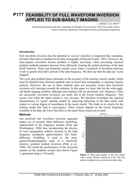
1P177 FEASIBILITY OF FULL WAVEFORM INVERSIONAPPLIED TO SUB-BASALT IMAGINGL. SIRGUE 1 , R. G. PRATT 21Ecole Normale Supérieure de Paris, Laboratoire de Géologie, 24 rue Lhomond, 75231 Paris Cedex, France.2Queen’s University, Department of Geological Sciences and Geological EngineeringIntroductionFull waveform inversion has the potential to recover velocities at migration-like resolution,far better than that of standard travel-time tomography (Pratt and Goulty, 1991). However, theleast-squares waveform inverse problem is highly non-linear, often preventing classicalgradient methods (steepest descent) from efficiently locating the global minimum of the datamisfit function. These non-linearities mainly occur when a mismatch of traveltime betweenevents is greater than half a period of the data frequency. We then say than the data are “cycleskipped”.The cycle skip problem places demands on the accuracy of the starting velocity model, whichmust be obtained from classical methods such as travel time tomography or stacking velocityanalysis. However, the use of these methods does not necessary assure that waveforminversion will converge towards the solution. In this paper we show that for the wide-angle,sub-basalt imaging problem, although tests starting with an unrealistic, low frequency (3Hz)are successful, waveform inversion can easily fail at the lowest realistic frequency. Thisoccurs even when the macro model is very accurate. We therefore investigate the requiredcharacteristics of “good” starting models by analyzing behaviour of the data misfit withrespect to various degree of smoothness in the macro model. This leads us to criteria for thestarting model that lead to convergence. These criteria depend on the lowest frequencyavailable in the data; the lower this limit is, the easier these criteria are to meet.MethodsOur preferred full waveform inversion approachmakes use of acoustic finite difference modelling,implemented in the frequency domain (Pratt andWorthington, 1990) thus incorporating the physicsof wave propagation without recourse to the highfrequency asymptotic approximation. The finitedifferencemodelling is used in the propagation/backpropagationsteps of a linearised,iterative, gradient method inversion (Pratt et al.,1996). We tested the performance of the inversionscheme on the synthetic seismic data shown Figure1, generated using a 1-D model.Figure 1: Shot point gather in the true modelwith a source Ricker centred on 4 Hz. The freesurface multiples are not present in these data.EAGE 64th Conference & Exhibition — Florence, Italy, 27 - 30 May 2002

2InversionFigure 2 shows the result of a successful inversion test, in which we initiated the inversion at3 Hz (an admittedly unrealistic low frequency); in this case we find ourselves in the basin ofattraction of the global minimum. Provided this condition is met, the frequency domainapproach turns out to be particularly appropriate since it allows one to recover a continuouswavenumber coverage of the model with only 3 frequencies (3,4.5,and 7.5 Hz) (Sirgue andPratt, 2001).However, when we initiate the inversion at 5 Hz, the inversion fails to converge towards thesolution. The inversion fails to locate the sediment-basalt discontinuity at 2.5 km depth;instead the reconstruction creates a strong oscillation in velocity with depth. This oscillationoccurs in spite of the fact that the starting model (the “macro model”) contains the correct lowwavenumber components. Thus, the initial model is not accurate enough to begin a fullwaveform inversion at 5 Hz.We suggest that the convergence difficulty may be mitigated adopting a layer strippingstrategy. This approach consists in reducing the kinematic error of events from deeper parts ofthe model by first solving for the shallow part of the model, thus reducing the risks of cycleskipping. A suitable strategy is to decompose the model into sediment, the basalt, and the subbasaltlayers. However, some convergence difficulties remain and we propose to study thetopography of the misfit function with various degrees of smoothness of the starting model.Layer stripping and data misfit functionWe constructed a suite of models (Figure 4) and tested the evolution of the least-squares dataFigure 2: Successful waveform inversion resultafter inverting sequentially 3, 4.5 and 7.5 Hzshowing the true model (grey), the starting model(dashed), the result after 3 Hz (dotted) and after3,4.5 and 7.5 Hz (solid).Figure 3: A failed waveform inversion resultafter inverting only 5 Hz data. See Figure 2 forcurve legend.

3misfit function. Preliminary tests (not shown) led us to conclud that it is an categoricalrequirement that the sediment-Basalt interface should be discontinuous and located at anaccurate depth: the reflected and refracted data from the basalts are highly non-linear withrespect to the location and nature of the top basalt interface.Figure 5 depicts the data misfit function as the three layers in the true model are decreasinglysmoothed (i.e., the high wavenumbers are progressively introduced), starting in each casefrom a quasi-homogeneous medium. An increase followed by a decrease of the misfitfunction is evidence of the presence of a local minimum. We conclude from Figure 5 that theuse of 3 Hz data would set few conditions on the starting model. In contrast, in order to obtainconvergence within the sediment layer when using frequencies 5 and 7 Hz, we evidentlyrequire a more accurate starting model, since the topography of the misfit function is likely toguide the waveform inversion into a local minimum. A starting model for the sediments, atthese frequencies would need to come from the region of Figure 5a) in which the misfit isdecreasing. In contrast, Figure 5b) suggests that a less accurate (i.e., more smooth) startingmodel would suffice.One should however be cautious about misleading conclusions for the sub-basalt layer whenexamining Figure 5c). Although the results for 5 and 7 Hz show a constant decrease in themisfit functions, these curves are nevertheless extremely flat. In other words, the misfitfunctions show very little sensitivity to the low and intermediate wavenumber components ofthe model. We suggest that this is because of the fact that only narrow incidence anglesilluminate the sub-basalt sediment.These results lead us to suggest a design for the profile of an adequate starting modela) b) c)Figure 4: Velocity models illustrating the “ideal” layer stripping strategy showing the true model (black)and the true model increasingly smoothed (gray) for a) the sediment, b) the basalt only and c) the subbasaltonly.a) b) c)Figure 5: Misfit functions of 3,5 and 7 Hz as the true model is decreasingly smoothed as shown Figure 4 fora) the sediment and the top of the basalt, b) the basalt only, c) the sub-basalt only.EAGE 64th Conference & Exhibition — Florence, Italy, 27 - 30 May 2002

4candidate for the waveform inversion at 7 Hz (Figure 6). The sediment layer needs strong apriori information on the low and intermediate wavenumbers, whereas the smoothnessrequirements of the velocities within the basalt are less demanding. The top and bottom of thebasalt must be discontinuous and located at the correct depth. Finally, the sub-basalt velocitiesrequire even higher wavenumber information than the sediments.ConclusionWe have identified some of the difficulties of waveforminversion applied to the sub-basalt imaging problem in anoptimistic context where a layer stripping strategy is feasible.We found that the basalt interfaces should remain reasonablydiscontinuous and located at an accurate depth. The inverseproblem is quite linear up to 3 Hz but some more stringentconditions are required in order to start an inversion fromfrequencies of 5 or 7 Hz. In these cases, some strong a prioriinformation is needed in the form of an accuratesediment/basalt interface model, and a very good estimationof the vertical gradient within the sediment and sub-basaltlayers. The basalt layer is less demanding thanks to strongdiving wave information.The vertical gradient within the sediment may be recoveredby stacking velocity analysis or travel time tomography.However, intra basalt reflections are often difficult to identifyFigure 6: True model (grey) and“ideal” starting model (black) foran inversion starting at 7 Hz.and prevent stacking velocity analysis. Nevertheless, strong diving waves at far offsets mightallow the use of travel time tomography to recover the low and intermediate wavenumbercomponents within the basalt layer.The highest degree of difficulty is likely to be encountered when solving for the sub-basaltlayer, even in the case where the velocities are perfectly known down to the base of the basalt.The lack of coherent events in the data coming from the sub-basalt effectively prevents anydetermination of the macro model in this area of the model. Moreover, since only narrowangles illuminate the sub-basalt target, waveform inversion will only be able to provide amigration like image of the sub-basalt sediments.AcknowledgmentWe thank CGG and the Geoscience Research Centre of TotalFinaElf for supporting this work.ReferencesPratt, R. G. and Worthington, M.H., 1990, Inverse theory applied to multi-source cross-holetomography: Part 1: Acoustic-wave equation method. Geophysical Prospecting, 38, 287-310.Pratt, R.G., and Goulty, N.R., 1991. Combining wave equation imaging with traveltimetomography to form high resolution images from crosshole data. Geophysics, 56, 208-224.Pratt, R. G., Song, Z.-M., Williamson, P., Warner, M., 1996, Two-dimensional velocitymodels from wide-angle seismic data by wavefield inversion, Geophys. J. Int., 124, 323-340.Sirgue, L., Pratt, R. G., 2001, An optimal choice of temporal frequencies for imaging:application to waveform inversion, 71 st Annual Meeting of the SEG, San Antonio