PDF Document - Clarkson University

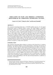
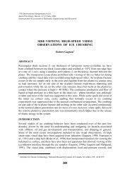
AE/ME 201 – Spring 2005100. reR is the relative error and has no units.( ±eR)± reR% = 100(3)RThe relative error changes with R because the eR isfixed for this experiment. Watch out if the denominatorever became zero. Small denominators havelarge relative error.Part 2 – Differential AmplifierIn this section, the Wheatstone bridge circuit willbe replaced with a differential amplifier.1. Connect the circuit as shown in Figures 6 (Endstations) or 7 (Middle station).Figure 5: Circuit diagram for part 1 (Middle stations)– From: it Hampden Model H-IT-2 Teacher’sManual, (1995) Hampden Engineering Corporation,pp. 2-20% Specify the absolute uncertaintyeR = 0.05; % [ Ohms ]eR = eR.*ones(size(R)); % [ Ohms ]% Compute the relative uncertaintyreR = 100.*eR./R;% Open a new figure windowfigure% Plot the data with error barserrorbar(x,R,eR,’ko’)% Add axis labels to the plotxlabel(’Displacement [ in. ]’)ylabel(’LVRT Resistance [ \Omega ]’)% percentThis is for symmetric error bars. eR is the absoluteerror and has engineering units.The percentage error is a relative error timesFigure 6: Circuit diagram for part 2 (End stations)– From: it Hampden Model H-IT-2 Student Manual,(2002) Hampden Engineering Corporation, pp.602. Reset the micrometer to its fully retracted position.3. Powering the Amplifier – The operation ofa simple transitor requires three power connectionsto the three materials (PNP or NPN).These connections set the field potential ofeach material and a voltage difference acrossthe two interfaces of the semiconductors. The4

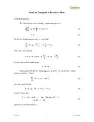
AE/ME 201 – Spring 2005Figure 9: Circuit diagram for balancing the amplifier(Middle stations) – From: it Hampden ModelH-IT-2 Teacher’s Manual, (1995) Hampden EngineeringCorporation, Appendix A6. Use the micrometer to displace the LVRT shaftby 0.100 inches. Record the voltage output bythe amplifier and increase the displacement byanother 0.100 inches. Continue until the displacementis equal to 1.000 inches and then decreasethe displacement to obtain an unloadingcurve.Data Analysis Notes:The resistance is calculated from the differential operationalamplifier equation. From the textbooksection on operational amplifiers, using V for voltageinstead of E, and the numbering of is replaced(1 is the inverting input)V out = (V in,2 − V in,1 ) R fR m(4)For your circuit, the input to the non-inverting inputis 0 volts and the feedback resistance is the linearvariable resistor. The input resistance of theinverting port is 15,000 ohms and the amplifier outis measured relative to 0V. ThenorV out = −V in,1R fR m(5)( Rin)R f = − V out (6)V in,1You should know the input voltage (about -15 V) orthe negative of the channel A power supply voltagethat was set and measured. Then feedback resistance(of the linear variable resistor) is calculated.Error PropagationSince resistance is calculated and not measured, theerror on the voltage is propagated to the resistancecalculation. Similar to differential calculus, assuminga fixed value for input quantities, the ’e’ actslike a differential operator and is written eV insteadof dV.( Rin)± eR f = ±eV out (7)−V in,1The precision interval on the voltmeter is ±1/2 thescale of the voltmeter. For example, if the voltmeterrange was set such that output voltage was 0.203volts, then the voltmeter increment was 0.001 voltsand the precision interval is ±0.0005 volts. Thenthe resistance error is (for 15.00V channel A)( 15kΩ)± eR f = ±0.5mV = ±0.5Ω (8)15VThen the precision interval for R is used to plot errorbars on the (x,R) plot for part 2. The part 1 andpart 2 curves are on the same plot and each curvehas error bars. This allows direct comparison. Notethat the x=0 reference for the micrometer must bethe same for both curves to make a proper comparison.Otherwise, the ’intercept’ does not match andthe curves may appear shifted.Tasks:1. Calculate the precision intervals for your measurementsin both the loading and unloadingcases. What is the percent error for each measurand?Does this make sense? What are otherpossible sources of error?2. Produce upscale and downscale plots for resistancemeasured using the decade box and positionmeasured from the micrometer. Is thereany hysteresis apparent in your measurements?If so, why?3. Calculate the feedback resistance from the measuredoutput voltage and the known input voltage.4. Calculate error bars for the computed feedbackresistances.5. For the same micrometer positions, comparethe length transducer resistance(from the wheatstone bridge experiment)to the calculated feedback resistance. Plot(x,y)=(wheatstone bridge R, calculated feedbackR). What would you expect the slope ofthis line to be, and do your results agree withyour expectations? If not, why not?References:1. Figliola, R.S., and Beasley, D.E., (2000) Theoryand Design for Mechanical Measurements, 3 rdEdition, John Wiley & Sons, Inc., New York, NewYork, USA, Chapter 6 & 126