Full-Reference Video Quality Assessment by Decoupling Detail ...

1100 IEEE TRANSACTIONS ON CIRCUITS AND SYSTEMS FOR VIDEO TECHNOLOGY, VOL. 22, NO. 7, JULY 2012Full-Reference Video Quality Assessment byDecoupling Detail Losses and Additive ImpairmentsSongnan Li, Student Member, IEEE, Lin Ma, Student Member, IEEE, and King Ngi Ngan, Fellow, IEEEAbstract—Video quality assessment plays a fundamental role invideo processing and communication applications. In this paper,we study the use of motion information and temporal humanvisual system (HVS) characteristics for objective video qualityassessment. In our previous work, two types of spatial distortions,i.e., detail losses and additive impairments, are decoupled andevaluated separately for spatial quality assessment. The detaillosses refer to the loss of useful visual information that will affectthe content visibility, and the additive impairments representthe redundant visual information in the test image, such as theblocking or ringing artifacts caused by data compression and soon. In this paper, a novel full-reference video quality metric isdeveloped, which conceptually comprises the following processingsteps: 1) decoupling detail losses and additive impairments withineach frame for spatial distortion measure; 2) analyzing the videomotion and using the HVS characteristics to simulate the humanperception of the spatial distortions; and 3) taking into accountcognitive human behaviors to integrate frame-level qualityscores into sequence-level quality score. Distinguished from moststudies in the literature, the proposed method comprehensivelyinvestigates the use of motion information in the simulation ofHVS processing, e.g., to model the eye movement, to predictthe spatio-temporal HVS contrast sensitivity, to implement thetemporal masking effect, and so on. Furthermore, we alsoprove the effectiveness of decoupling detail losses and additiveimpairments for video quality assessment. The proposed methodis tested on two subjective quality video databases, LIVE and IVP,and demonstrates the state-of-the-art performance in matchingsubjective ratings.Index Terms—Human visual system (HVS), spatial distortionsdecoupling, video quality assessment.I. IntroductionDEMANDS for various kinds of video services, such asdigital TV, IPTV, video on demand, video conference,video surveillance, and so on, boom with the advances in videoprocessing and communication technologies. A typical videoservice chain consists of sequential components, e.g., acquisition,enhancement, compression, transmission, transcoding, reconstruction,restoration, presentation, and so on, implementedby software and hardware systems. Video quality assessment(VQA) plays a central role in the life cycle of most of thesesystems: from the system design, performance evaluation, toManuscript received June 16, 2011; revised October 7, 2011; acceptedDecember 11, 2011. Date of publication March 9, 2012; date of current versionJune 28, 2012. This paper was recommended by Associate Editor E. Magli.The authors are with the Department of Electronic Engineering, The ChineseUniversity of Hong Kong, Shatin, Hong Kong (e-mail: snli@ee.cuhk.edu.hk;lma@ee.cuhk.edu.hk; knngan@ee.cuhk.edu.hk).Color versions of one or more of the figures in this paper are availableonline at http://ieeexplore.ieee.org.Digital Object Identifier 10.1109/TCSVT.2012.21904731051-8215/$31.00 c○ 2012 IEEEthe in-service functionality monitoring. In system design, anobjective VQA algorithm can work online to bring benefitsincluding performance improvement and/or resource saving;in performance evaluation, customer-oriented VQA can beemployed to compare performances of competing systems,e.g., two different video coding schemes; for in-service qualitymonitoring, VQA continuously evaluates the system outputs,troubleshoots when system failure occurs, so as to guaranteehigh quality video service delivery. Since the human visualsystem (HVS) is the ultimate receiver of the video service,subjective VQA (subjective viewing test) is considered to bethe most reliable way to evaluate visual quality. Its applicationsinclude assessing visual systems, benchmarking objectiveVQA algorithms, and so on. However, subjective VQA is notfeasible for online manipulations, which makes it impracticalfor system design and quality monitoring. Furthermore, inorder to ensure repeatable and statistically meaningful results,subjective VQA should precisely follow the standards [2]–[4]to set up the viewing environment, and should employ sufficientsubjects in the viewing tests to account for individualdifferences. Satisfying these requirements makes subjectiveVQA time-consuming and expensive. Therefore, an accurateobjective VQA algorithm, or namely video quality metric(VQM), becomes of paramount importance to the developmentof future video processing and communication applications.The obstacle to an accurate VQM comes from numerousaspects: 1) the input video signal contents are diverse (e.g.,sports, animations, movies, news report) creating problems,such as unpredictable visual attention, and so on; 2) visualsystems generate various spatial artifacts (e.g., blocking, ringing,blurring, white noise) and/or temporal artifacts (e.g., jitter/jerkymotion), which may be compounded during the videodelivery; 3) the viewing conditions, such as the environmentlightness, the display type and calibration, the viewing distance,and so on influence the distortion visibility; 4) the HVSis extremely complex and seems impossible to be completelymodeled in the near future; and 5) visual quality judgmentis viewer dependent, related to unpredictable factors such asthe viewer’s interests, expectation, quality experience, and soon. Consequently, VQM is not expected to be unconditionallyas accurate and reliable as the subjective VQA. Instead, it istypical for most VQMs to restrict their utilities to specific setsof input contents, artifacts, and viewing conditions.It is customary to classify VQM into three categoriesaccording to the reference availability: full-reference (FR),reduced-reference (RR), and no-reference (NR) metrics. In

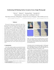
LI et al.: FULL-REFERENCE VIDEO QUALITY ASSESSMENT 1101FR metrics, the reference is fully available and is assumedto have maximum quality. They can be applied in systemdesign and performance evaluation. For instance, in lossyvideo coding, the coding tools (e.g., intra and interprediction,transformation, quantization, de-blocking filter) and thecoding modes (e.g., various intra or intermodes) are chosenaccording to their abilities to optimize rate and distortion, thelatter of which can be quantified by FR metrics due to theavailability of the reference. In watermarking, performancesof various schemes are evaluated based on three majorfactors: robustness (to malicious attack), capacity (to embedinformation), and distortion perceptibility, where the distortionperceptibility can be measured by FR metrics. RR metricsextract features from the reference video, transmit them to thereceiver side (by an ancillary channel [5] or by watermarking[6]) to compare against the corresponding features extractedfrom the distorted video. The design of RR metric mainlytargets at quality monitoring. These features should becarefully selected to achieve both effectiveness and efficiency,i.e., predicting quality with great accuracy and small overheadfor feature representation. NR metrics require no reference,therefore are most broadly applicable. For many inherentlyno-reference applications, such as video signal acquisition,enhancement, and so on, NR metric is their only choice foronline quality assessment. Not surprisingly, NR metric designis tough, facing challenges of limited input information.Therefore, to guarantee acceptable prediction performance,many NR metrics are designed to cope with specific artifacts,such as blocking, blurring, ringing, jitter/jerky motion, andso on, scarifying versatility for prediction accuracy. For acomprehensive overview on NR metrics, please refer to [7].In this paper, we propose a novel FR VQM. It promotes andcompletes our preliminary work [40] by extensively exploringthe motion information and HVS temporal characteristics forvideo quality assessment. For spatial distortion measurement,we adopt the method [1] previously proposed by the authorsfor image quality assessment, i.e., separately evaluating detaillosses and additive impairments which are decoupled from theoverall spatial distortions. In Section II-A, we briefly overviewFR image quality metrics (IQM) and explain in more detailthe adopted spatial distortion measurement. In the followingsteps, we simulate the HVS processing, more specifically, howthe human beings perceive the spatial distortions, using severalmajor HVS characteristics, such as contrast sensitivity function(CSF), visual masking, information pooling, and so on. Comparedwith our preliminary work [40] in which motion informationof the video was not considered and with most previousstudies, the contribution of the proposed VQM comes fromthe extensive use of motion information to simulate the HVSprocessing, that is, motion vectors are derived in the waveletdomain, and employed in the eye-movement model, the spatiovelocityCSF, the motion-based temporal masking, and so on.We also simulate cognitive human behavior, which originallywas proposed to be used in continuous quality evaluations[37], [38], and have proved its effectiveness in sequence-levelquality prediction. In Section II-B, an introduction is givenon how the previous VQMs use motion information and HVScharacteristics for video quality assessment. The major differencesbetween them and the proposed VQM are discussedin more detail. Section III elaborates the proposed VQM.Section IV shows the experimental results using both standarddefinitionand high-definition video databases to illustrate theperformance of the proposed VQM in matching subjectiveratings. Section V provides the conclusion.II. BackgroundA. Full-Reference Image Quality AssessmentMost FR IQMs are general-purpose, that is, being able tohandle various artifacts. As pointed out in [8], this crossartifactversatility is crucial for benchmarking image processingsystems. Pixel-based metrics, such as MSE/PSNR and soon, correlate visual quality with pixel value differences. Asproved in many studies, MSE/PSNR predicts quality of whitenoisedistorted images with excellent accuracy, but failed tocope with other distortion types and cross-artifacts qualitymeasurement. HVS-model-based metrics, such as those in[9]–[12], employ HVS models to simulate the low-level HVSprocessing of the visual inputs. They are often criticized, e.g.,in [13], because these HVS models may be unsuitable forsupra-threshold contrast measure and show a lack of geometricmeaning [14, Fig. 4]. High-level HVS processing mechanismstill cannot be fully understood. Therefore, many recent IQMssimply make use of common knowledge or assumption aboutthe high-level HVS characteristics to guide quality prediction.For example, it is well acknowledged that structural informationis critical for cognitive understanding; hence, the authorsof [14] made the assumption that the structure distortion is agood representative of visual quality variation. They proposedthe structure similarity index (SSIM) which distinguishesstructure distortions from luminance and contrast distortions.This assumption has been well recognized and applied in otherIQMs [8], [15], [16]. Another well-known assumption madeby the authors of the visual information fidelity criterion (VIF)[17] is that the HVS correlates visual quality with the mutualinformation between the reference and distorted images. Themutual information resembles the amount of useful informationthat can be extracted from the distorted image. AlthoughVIF seems to be quite different from SSIM in terms of thefundamental assumption, down to the implementation, the twoIQMs share similarities, as analyzed in [18].In this paper, we adopt our previous work [1] to measurethe spatial distortions. Instead of treating the spatial distortionsintegrally, they are decomposed into detail losses and additiveimpairments. As the name implies, detail losses refer to theloss of useful information which affects the content visibility.Additive impairments, on the other hand, refer to the redundantvisual information which does not belong to the originalimage. Their appearance in the distorted image will distractviewer’s attention from the useful picture contents, causingunpleasant viewing experience. To assist understanding, anillustration is given in Fig. 1. In Fig. 1(a), the distorted imageis separated into the original image and the error image.Typically, HVS-model-based IQMs will try to simulate lowlevelHVS responses to the error image, treating these errors ina similar way. As shown in Fig. 1(b), the proposed method will

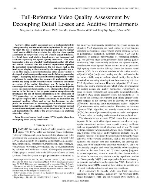
1102 IEEE TRANSACTIONS ON CIRCUITS AND SYSTEMS FOR VIDEO TECHNOLOGY, VOL. 22, NO. 7, JULY 2012Fig. 1. Example of (a) separating the distorted image into the original imageand the error image, (b) separating the error image into the detail loss imageand the additive impairment image, and (c) separating the distorted image intothe restored image and the additive impairment image.further separate the image errors into detail losses and additiveimpairments. For JPEG compressed images, as the one shownin Fig. 1, the detail loss is caused by DCT coefficientsquantization, and the additive impairment mainly appears to beblocky. In our implementation, we first separate the distortedimage into an additive impairment image and a restored image,as shown in Fig. 1(c). The restored image exhibits the sameamount of detail losses as the distorted image but is additiveimpairment free. And then, the detail loss can be obtained bysubtracting the restored image from the original one.B. Exploiting Temporal Information for Video QualityAssessmentIn comparison to images, videos involve one more dimensionwhich apparently will render quality prediction moredifficult. The predictive performance of the state-of-the-artVQMs measured by correlation coefficient is around 0.8typically [19], while on the other hand for the state-of-theartIQMs this value on most databases is above 0.9 [1]. Tomake video quality prediction more precise, besides accuratelymeasuring the spatial distortions, motion information of thevideo and temporal characteristics of the HVS should be fullyinvestigated.A frequently used method of exploiting temporal HVScharacteristics is to decompose the video signal into multiplespatio-temporal frequency channels and then assign differentweights to them according to, e.g., the CSF. It is believedthat the early stage of the visual pathway separates visualinformation into two temporal channels: a low-pass channeland a band-pass channel, known as the sustained and transientchannels, respectively. Several VQMs model this HVS mechanismby filtering the videos along the temporal dimensionusing one 1 or two filters. Recently, Seshadrinathan et al. [19]proposed to use 3-D Gabor filters to decompose the videolocally into 105 spatio-temporal channels enabling the calculationof motion vectors from the Gabor outputs. Different fromthe typical CSF weighting, in [19] each channel is weightedaccording to the distance between its center frequency and aspectral plane identified by the motion vectors of the referencevideo. Lee et al. [20] proposed to find the optimal weights forchannels by optimizing the metric’s predictive performance onsubjective quality video databases.Masking is another visual phenomenon critical for videoquality assessment. The visibility of distortions is highly dependenton both the spatial and temporal activities. However,most VQMs take into account only the spatial masking effect[19], [21]–[24]. And although temporal masking is involvedin a few studies [25]–[27], motion vectors approximating theeye tracking movement are rarely investigated. Lukas et al.[25] used the derivative of the outputs of a spatial visualmodel along the time axis to measure the local temporalactivities, which then serves as input to a nonlinear temporalmasking function. This function was calibrated by fittingpsychophysical data. Lindh et al. [26] extended a classical divisivenormalization-based masking model [28] from spatial tospatio-temporal frequency domain. Chou et al. [27] proposedto measure temporal activity simply by calculating pixel differencesbetween adjacent frames. They constructed a temporalmasking function via specifically designed psychophysicalexperiment. Chen et al. [29] conducted experiments to refinethis function. Similar temporal masking functions were takenby a host of video quality metrics and JND models [30]–[33].High-level temporal characteristics of the HVS can beused in the pooling process. Pooling models the informationintegration which is believed to happen at the late stage ofthe visual pathway, and usually it is carried out by summationover all dimensions to obtain an overall quality score for animage or video. Wang et al. [34] used relative and backgroundmotions to quantify two terms: motion information content andperceptual uncertainty, which in the next step were used asweighting factors in the spatial pooling process. In TetraVQM[35], a degradation duration map is generated for each frameby analyzing the motion trajectory, and serves as a weightingmatrix in spatial pooling. Ninassi et al. [36] proposed to takeinto account the temporal variation of spatial distortions in thetemporal pooling process. In [24], [37], and [38], the authors1 For computational simplicity, only the sustained channel is isolated.

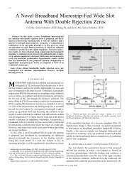
LI et al.: FULL-REFERENCE VIDEO QUALITY ASSESSMENT 1103Fig. 2.Systematic framework of the proposed VQM.considered the asymmetric human behavior in responding toquality degradation and improvement.In this paper, three HVS processing simulation modules,i.e., the eye movement spatio-velocity CSF, the motion-basedtemporal masking, and the asymmetric temporal pooling, aredeployed to extend our IQM [1] into the state-of-the-art VQM.Daly’s eye movement spatio-velocity CSF [39] which modelsHVS sensitivity as a function of the spatial frequency and thevelocity of the visual stimuli is used for the first time in videoquality prediction. Compared to the other CSF models, Daly’smethod gives us mainly two advantages: 1) a more accurateCSF modeling; and 2) the involvement of the eye movementwhich is common in natural viewing conditions. We alsopropose a novel temporal masking method which differs fromthe most existing ones in the use of the motion information.The asymmetric temporal pooling method is directly adoptedfrom [24] with the parameters tuned on a training set.III. Proposed MethodA. FrameworkThe framework of the proposed VQM is illustrated inFig. 2. It consists of several sequential processing modules. Ingeneral, for each frame of the distorted video, the distortionswithin are separated into additive impairments and detaillosses. Motion-based contrast sensitivity function and visualmasking are incorporated to rectify the intensities of theimpairment images so that the intensity values become betterrepresentative of the low-level neural responses of the HVS.The influences of additive impairments and detail losses tovisual quality are independently evaluated, and then combinedtogether by weighted summation to generate quality score foreach frame. An overall quality score indicating the qualityof the whole video sequence is derived by temporal poolingover the individual quality scores of the video frames. Detailedinformation on each processing module and the meaning of thenotations in Fig. 2 will be given below. It should be noted thatthe proposed VQM works with luminance only. Color inputswill be converted to gray scale before further processing.B. Decoupling Additive Impairments and Useful ImageContentsAs introduced in Section II-A, in our VQM each distortedvideo frame (d n , indexed by time n) is separated into anadditive impairment image and a restored image, which isexemplified in Fig. 1(c). The decoupling algorithm whichperforms in the critically sampled wavelet domain is adoptedfrom our previous work [1]. To reduce its computationalcomplexity, two modifications are applied: 1) the original db2wavelet transform is replaced by the simpler Haar wavelettransform; and 2) since it rarely happens in practical videoapplications, contrast enhancement is not distinguished fromspatial distortions as in [1]. The derivation of the decouplingalgorithm used in this paper is given below.In the following context, o, d, r, a are used to represent theoriginal, distorted, restored, and additive impairment images,respectively. Our intention is to get the restored image r whichexhibits the same amount of detail losses as the distortedimage d but is additive impairment free. After calculating r,the additive impairment image a can be obtained by a = d−r.as shown in Fig. 1(c).The restored image r consists of local image patches r iwhere i indicates the local position. Each patch r i can befurther decomposed into multiple components of differentspatial frequenciesS∑r i = r s i (1)s=0where s indicates the nominal spatial frequency. Such decompositionwhich requires both time and frequency localizationof the signal can be implemented by wavelet transform.Therefore, r s i can be considered as the image component reconstructedfrom the wavelet coefficients of subband s aroundlocation i. The decomposition is applied to the original imageo and the distorted image d to derive o s i and ds i , respectively. Tomake r s i additive impairment free, the gradient of rs i should beproportional to that of o s i , i.e., ∇rs i = ks i ×∇os i , where the valueof ki s is limited to [0,1] to account for the detail losses. For highfrequency subbands (s ∈{1, 2, ..., S}), the mean values of r s iand o s i are equal to zero. Therefore, to satisfy the requirementson ∇r s i , we impose that rs i = ks i × os i .Another objective of the decoupling is to make r s i exhibitthe same amount of detail losses as d s i . The distorted imagepatch d s i can be taken as the composite of two signals,i.e., the useful image content and the additive impairments.Since the additive impairments correlate poorly with r s i ,asexemplified by Fig. 1(b), the similarity between r s i and d s iis approximately equivalent to the similarity between r s i andthe useful image content of d s i . Therefore, making rs i exhibitthe same amount of detail losses as d s i (i.e., maximizing thesimilarity between r s i and the useful image content of d s i )can be achieved equivalently by maximizing the similaritybetween r s i and d s i . For computational simplicity, the imagesimilarity is measured by the sum of squared differences:min k si ∈[0,1]||r s i − ds i ||2 . Given an orthonormal discrete wavelettransform (DWT), the following equations hold:min k si ∈[0,1] ||r s i − ds i ||2= min k si ∈[0,1] ||DWT [r s i − ds i ]||2= min k si ∈[0,1] ||DWT [ki s × os i − ds i ]||2 (2)= min k si ∈[0,1] ||ki s × DWT [os i ] − DWT [ds i ]||2= min k si ∈[0,1] ||ki s × Os i − Ds i ||2

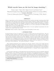
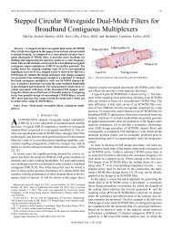
1104 IEEE TRANSACTIONS ON CIRCUITS AND SYSTEMS FOR VIDEO TECHNOLOGY, VOL. 22, NO. 7, JULY 2012Fig. 3. Subband indexing. Each subband is indexed by a level and anorientation {λ, θ}. θ = 2, 3, and 4 denote the vertical, diagonal, and horizontalsubbands, respectively.where O s i and D s i denote the DWT coefficients of o s i and d s i ,respectively. The closed-form solution of the scale factor ki s in(2) can be given by( < Oski s = clip i · D s i > )||O s , 0, 1(3)i ||2where < · > denotes the inner product operation, andclip(x, 0, 1) is equivalent to min(max(0,x), 1). According tothe size of the local image patch, O s i and D s i can be avector of DWT coefficients or just a single DWT coefficient.We found experimentally that the patch size is inessentialto the decoupling performance. Therefore, for computationalsimplicity we use a single DWT coefficient to represent O s iand D s i . In this way, (3) is simplified to be the division of twoscalar values.In the following discussion, n is used to index each frame,{λ, θ} is used to index each wavelet subband, as illustratedin Fig. 3, and {i, j} is used to index the DWT coefficientposition. A four-level Haar DWT is applied to the original (o n )and distorted (d n ) frames, generating the DWT coefficientsO n (λ, θ, i, j) and D n (λ, θ, i, j), respectively. Based on theabove analysis, scale factors of the high frequency subbandscan be given by()D n (λ, θ, i, j)k n (λ, θ, i, j) =clipO n (λ, θ, i, j)+10 , 0, 1 (4)−30where the constant 10 −30 is to avoid dividing by zero. Sinceintuitively the original mean luminance cannot be recoveredfrom the distorted frame, the approximation subband of therestored image is made to equal that of the distorted one. Eventually,the DWT coefficients of the restored image R n (λ, θ, i, j)can be obtained by{Dn (λ, θ, i, j), θ =1R n (λ, θ, i, j) =k n (λ, θ, i, j) × O n (λ, θ, i, j), otherwise(5)where θ = 1 indicates the approximation subband. Since DWTis linear and a = d − r, DWT coefficients of the additiveimpairment image can be calculated byA n (λ, θ, i, j) =D n (λ, θ, i, j) − R n (λ, θ, i, j). (6)C. Motion EstimationMotion estimation (ME) algorithms aim at finding motionvectors representing object trajectory. In video compression,motion vectors can be used to remove the interframe redundancy.In video quality assessment, as will be elaboratedbelow, the motion of the visual stimuli affects the HVS sensitivity.The use of motion vectors can enhance the modelingaccuracy of how the HVS perceives distortions. As shownin Fig. 2, the ME is performed in the wavelet domain ofthe original video sequence. Wavelet transform decomposes avideo frame into subbands of different resolutions. The motionvectors of these multiresolution subbands are highly correlatedsince they actually specify the same motion structureat different scales. Therefore, Zhang et al. [41] proposed awavelet domain multiresolution ME scheme, where motionvectors at higher resolution are predicted by the motion vectorsat the lower resolution and are refined at each step. Theproposed method not only considerably reduces the searchingtime, but also provides a meaningful characterization of theintrinsic motion structure. We directly adopt Zhang’s schemeto perform the wavelet domain ME. Specifically, the motionvectors V λ,θ for the coarsest subbands (λ =4,θ =1, 2, 3, 4)are estimated by block-based integer-pixel full search witha search range of [−3, +3]. These motion vectors are thenscaled by V λ,θ =2 (4−λ) × V 4,θ (λ =1, 2, 3,θ =2, 3, 4), andused as initial estimates for the finer subbands. These initialmotion vectors are further refined by using full search witha relatively small search range [−2, +2]. The block size isadapted to the scale, i.e., 2 (5−λ) × 2 (5−λ) (λ =1, 2, 3, 4), sothat no interpolation is needed as the motion vectors propagatethrough scales. The motion vectors will be used in the contrastsensitivity function. The motion estimation errors, E n , are alsosaved for use in the temporal masking. It is worth noting thatthe critically sampled wavelet domain ME is not as accurate asthe spatial domain ME due to the shift-variant property causedby the decimation process of the wavelet transform. As willbe discussed below, we try to partially compensate the MEimprecision in the temporal masking process. More advancedwavelet domain ME algorithms can be used, but we foundZhang’s scheme a good compromise between performance andsimplicity.D. Contrast Sensitivity FunctionHuman contrast sensitivity is the reciprocal of the contrastthreshold, i.e., the minimum contrast value for an observerto detect a stimulus. It is related to the properties of thevisual stimulus, notably its spatial and temporal frequencies.A spatio-temporal CSF is a measure of the contrastsensitivity against spatial and temporal frequencies of thevisual stimulus. In the proposed method, we adopt Daly’seye movement spatio-velocity CSF model [39], as shownin Fig. 4, which was extended from Kelly’s spatio-temporalCSF model [42] by taking into account the natural drift,smooth pursuit, and saccadic eye movements. In natural viewingconditions, evaluating visual quality must involve eyemovements. Hence, incorporating eye movement model inthe VQM should help to boost its predictive performance.Furthermore, rather than using flickering waves, such as in [23]and [43], the derivation of Daly’s model is based on travelingwaves which better represent the natural viewing conditions[39], [44].

LI et al.: FULL-REFERENCE VIDEO QUALITY ASSESSMENT 1105g sp =0.82, v MIN =0.15, v MAX = 80. Given the magnitude,v, of the motion vector and the frame rate, f r , in frames persecond (f/s), the image plane velocity can be calculated asv I = 180 · h · 2λ · v · f r(11)π · d · f swhere the meaning of the notations is the same as (8). Using(7)–(11) and the motion vectors derived from the waveletdomain ME, for each wavelet coefficient a CSF value canbe calculated. As illustrated in Fig. 2, we simulate the CSFprocessing in the wavelet domain of the original image, thetwo decoupled images, and the ME prediction error image. Itis implemented by multiplying each wavelet coefficient withits corresponding CSF value. The resultant signals are denotedas O csfn, respectively., Rcsf n, Acsf n, Ecsf nFig. 4.Daly’s eye movement spatio-velocity CSF model.Daly’s model can be formulated asCSF(ρ, v R )=k · c 0 · c 1 · c 2 · v R · (c 1 2πρ) 2 exp(− c 14πρρ max)k = s 1 + s 2 ·|log(c 2 v R /3))| 3ρ max = p 1 /(c 2 v R +2)where ρ is the spatial frequency of the visual stimulus incy/deg and v R is the retinal velocity in deg/s. The values ofthe constants are consistent with that of [39], i.e., c 0 =1.14,c 1 =0.67, c 2 =1.92, s 1 =6.1, s 2 =7.3, p 1 =45.9. Since theyare not quite related to our subject, please refer to [39] forthe physical meanings of these constants. The nominal spatialfrequency of subbands in scale λ can be given byρ(λ) =π · f s · d(8)180 · h · 2 λwhere d is the viewing distance, h is the picture height, andf s is the cycles per picture height. The retinal velocity v R canbe calculated as follows:(7)v R = v I − v E (9)where v I is the image plane velocity, and v E is the eyevelocity. There are three types of eye movements modeled,i.e., the natural drift eye movements (0.8–0.15°/s) whichare responsible for the perception of static imagery duringfixation, the saccadic eye movements (160–300°/s) which areresponsible for rapidly moving the fixation point from onelocation to another, and the smooth pursuit eye movementswhich lies between the two endpoints and occur when the eyeis tracking a moving object. Adopted from [39], the equationused to model the eye velocity v E as a function of the imageplane velocity v I isv E = min⌊(g sp · v I )+v MIN ,v MAX ⌋ (10)where g sp is the gain of the smooth pursuit eye movementsmodeling the eye tracking lag, v MIN is the minimum eyevelocity due to drift, and v MAX is the maximum eye velocitybefore transmitting to saccadic movements. As in [39], we setE. Spatial and Temporal MaskingSpatial masking refers to the visibility threshold elevation ofa target signal caused by the presence of a superposed maskersignal. Traditional spatial masking methods use original imageto mask the distortions. However, artifacts may make the distortedimage less textured compared to the original, especiallyfor low-quality images where the contrasts of the texturesand edges have been significantly reduced. In our method,the restored image and the additive impairment image aredecoupled, as illustrated in Fig. 1(c). Since the two decoupledimages are superposed to form the distorted image, one’spresence will affect the visibility of the other. Therefore, in theproposed metric both images serve as the masker to modulatethe intensity of the other. As in [1], the equation used tocalculate the spatial masking thresholds is3∑T λ = m s × (|M λ,θ |⊗w) (12)θ=1where w isa3× 3 weighting matrix with the central elementbeing 1/15 and all the other elements being 1/30, |M λ,θ | is theabsolute value of the {λ, θ} wavelet subband of the maskersignal, ⊗ denotes convolution, and T λ is the threshold mapfor the three wavelet subbands in scale λ. The m s determinesthe slope of the masking function. As in [1], we set m s =1for all scales. We take the absolute value of the CSF-weightedwavelet coefficients of the maskee signal, i.e., |R csfn | (|Acsf n |),subtract from them the spatial masking thresholds given by(12) with A csfn (R csfn ) as the masker signal, and clip theresultant negative values to 0. After the spatial masking, thewavelet coefficients of the restored and additive impairmentimages are represented by R smn and A smn , respectively. Asshown in Fig. 2, Snsm which denotes detail losses is derivedby subtracting R smn from O csfn , i.e., the CSF-weighted waveletcoefficients of the nth original frame.As aforementioned in Section II, temporal masking is oftenmodeled as a function of temporal discontinuity, that is, thehigher the interframe differences, the stronger the temporalmasking effect. To the best of our knowledge, temporalmasking methods in the literature, such as the ones used in [27]and [30]–[33], measure interframe differences of the originalvideo sequence (o n − o n−1 ) as the masker to mask distortions,

1106 IEEE TRANSACTIONS ON CIRCUITS AND SYSTEMS FOR VIDEO TECHNOLOGY, VOL. 22, NO. 7, JULY 2012and notably they do not consider the eye movement. Asdiscussed above, the human eyes may track the motion. Hence,the use of interframe differences without taking into accountmotion vectors may exaggerate the temporal masking effect.In our implementation, the CSF-weighted ME prediction errorimage, Encsf , is used to calculate the temporal masker. In caseof inaccurate motion vectors as discussed in Section III-C,the temporal masker is given by min(Encsf , (Ocsf n − O csfn−1 )),which means that each element of the temporal masker equalsthe smaller one of the prediction error and the interframedifference. Equation (12) with the spatial masking factor m sreplaced by the temporal masking factor m t is used to calculatethe temporal masking thresholds. We set m t =0.4 by tuningthe predictive performance of the VQM on a training set, as tobe explained in Section IV. The masking process also followsthe aforementioned three steps: taking absolute value of themaskee, subtracting masking thresholds, and then clippingnegative values to zero. The temporal masker is used tomodulate the intensities of the two types of spatial distortions:the detail losses (Snsm ) and the additive impairments (Asm n ). Theresultant signals are denoted as Sntm and A tmn , respectively.F. Two Quality Measures and Their CombinationAs in [40], the additive impairment measure (AIM) and thedetail loss measure (DLM) are given byf AIMn =f DLMn =∑λ∑θ [∑ i,j∈center Atm n (λ, θ, i, j)2 ] 1/2θ ≠ 1 (13)N p∑∑λλ∑θ [∑ i,j∈center Stmn (λ, θ, i, j)2 ] 1/2∑θ [∑ θ ≠ 1 (14)i,j∈center Ocsf n (λ, θ, i, j) 2 ] 1/2where θ ≠ 1 means that we exclude the use of approximationsubband in the spatial pooling, and (i, j) ∈ center indicatesthat only the central region of each subband is used, whichserves as a simple region of interest model. Since additive impairmentsare relatively independent of the original content, weassume that visual quality with respect to additive impairmentscan be predicted by analyzing their intensities without consideringthe original content. On the other hand, visual qualitywith respect to detail losses is supposed to be connected withthe percentage of visual information loss. Therefore, in AIMand DLM the integrated distortion intensities are normalizedby the pixel number N p and an integrated value associatedwith the original content, 2 respectively.To derive the frame-level quality score, fnAIMcombined by weighted summation 3f n = f AIMnand f DLMnare+ w · f DLMn . (15)The weighting factor w is set to 2.47 × 10 3 by performancetuning, as to be explained in Section IV.2 To make complexity affordable, DLM only provides an approximatecalculation of the visual information loss.3 The typical value ranges of fnALM and fnDLM are from 0 to 600 and from0 to 0.3, respectively.G. Temporal PoolingIn temporal pooling, quality scores f n , n ∈{1, ..., N}, ofthevideo frames are integrated to yield the overall quality scoreof the whole video sequence. Rather than directly calculatingtheir average, preprocessing on the frame-level scores is performedto generate intermediate results f n ′ , n ∈{1, ..., N}. Thepreprocessing simulates several cognitive human behaviorsthat have been reflected in the results of many continuous qualityevaluations [37], [38], like the smoothing effect, i.e., thesubjective ratings typically demonstrate far less variation thanthe objective quality scores, and the asymmetric tracking, i.e.,the human observers are more sensitive to degradation thanto improvement in picture quality. We adopt the implementationin [24] which is a lowpass function of the frame-levelscores{ ′ff ′ n = n−1 + a −△ n , if △ n ≤ 0f ′ n−1 + a (16)+△ n , if △ n > 0where △ n = f n − f ′ n−1 . The value difference between a − anda + embodies the asymmetric tracking human behavior. In [24],the values of a − and a + are derived by training (a − =0.04 anda + =0.5). We re-tune the two parameters on our training set,and get similar results: a − =0.075, a + =0.431. This parametersetting is used in our VQM. Finally, the overall sequence-levelquality score s is given by averaging the intermediate resultsf n ′ , n ∈{1, ..., N}s = 1 N∑f ′ nN. (17)IV. ExperimentsA. Subjective Quality Video Databases and PerformanceEvaluation CriteriaIn this section, two subjective video databases are usedfor performance evaluation, i.e., the LIVE and IVP subjectivequality video databases. A subjective quality video databaseprovides each of its distorted video a subjective score, whichwas obtained through subjective viewing tests. To evaluatepredictive performance of a VQM, these subjective scorescan be used as the ground truths to be compared against themetric’s outputs. LIVE video database [45]–[47] consists of150 768 × 432p distorted videos generated from ten referencevideos of natural scenes with frame rates of either 25 or50 f/s. Four practical distortion types for standard-definitionvideos are involved: H.264 compression, MPEG-2 compression,transmission errors over IP networks, and transmissionerrors over wireless networks. IVP video database [48] isdeveloped by the author and his associates. It consists of128 1920 × 1088p distorted videos with frame rate of 25 f/s.The reference videos contain both natural scenes and animations.Four practical distortions for high-definition videos areinvolved: H.264 compression, MPEG-2 compression, Diracwavelet compression [49], and transmission errors over IPnetworks. Both databases pack their videos into YUV 4:2:0,and the duration of each distorted video sequence is around10 s. The reference and distorted videos are well spatiallyn=1

LI et al.: FULL-REFERENCE VIDEO QUALITY ASSESSMENT 1107and temporally registered, and there is no need for luminancechrominancealignment [50].As required by some performance measures, such as thelinear correlation coefficient, it is necessary to nonlinearlymap each metric output (objective score) x to Q(x), sothat Q(x) and the subjective scores approximately exhibit alinear relationship. We adopt the following nonlinear mappingfunction [17] for all VQMs in the experiments:(Q(x) =β 1 × 0.5 −)1+ β 4 × x + β 5 .1+exp(β 2 × (x − β 3 ))(18)The fitting parameters {β 1 ,β 2 ,β 3 ,β 4 ,β 5 } are determined byminimizing the sum of squared differences between themapped objective scores Q(x) and the subjective scores. As tobe introduced below, we divide the LIVE video database intoa training set and a test set. In the following experiments, thefitting parameters are determined on the training set and areused to evaluate the predictive performances of the VQMs onthe test set. As for the IVP video database, due to the limitednumber of test sequences, we do not divide it into a trainingset for determining the fitting parameters and a test set forthe evaluation. On the other hand, the fitting parameters arechosen and tested on the entire IVP database.The mapped scores Q(x) and the subjective scores serve asinputs to three performance measures: the linear correlationcoefficient (LCC), the root mean squared error (RMSE), theSpearman rank-order correlation coefficients (SROCC). Forformulation and detailed comparison between these performancemeasures, please refer to [1] and [51]. In general, higherLCC indicates stronger correlation between objective andsubjective scores, hence, better predictive performance; RMSEmeasures the predictive errors, so the smaller the RMSE thebetter the predictive performance. SROCC measures correlationbetween ranks of the objective and subjective scores,instead of their magnitudes as the LCC does. Therefore, it isimmune to a failed monotonous nonlinear mapping.B. ParameterizationThere are four parameters to be determined, i.e., m t , w,a − , and a + . We select 60 videos 4 from LIVE video databaseto train these parameters. The objective is to maximize theSROCC of the resultant VQM on this training set. In thetraining process, m t is changed from 0 to 0.9 in step of 0.1.For each m t , the best w is found by a global optimization algorithm,i.e., the genetic algorithm [52], with a − = 1 and a + =1(i.e., f ′ n =f n). Comparing all the {m t , w} pairs, {m t =0.4,w =2.47 × 10 3 } that maximizes the SROCC is chosen as thefinal parameters setting. Fig. 5 shows the m t training results.When m t =0.4, SROCC reaches the peak. Further increase ofm t will degrade the predictive performance, since the temporalmasking effect may be overestimated. After m t and w arefixed, a − and a + are found also by the genetic algorithm.Table I shows how the processing modules introduced inSection III accumulatively improve the predictive performance4 The 60 distorted videos are generated from four reference sequences, i.e.,Tractor, Sunflower, Mobile and Calendar, Park Run, randomly chosen fromthe LIVE video database.Fig. 5. Tuning results of the parameter m t .TABLE IAccumulative Performance Improvement (Evaluated bySROCC) of the Proposed VQMLIVE (Training) LIVE (Test) IVPDCP 0.7911 0.6639 0.4478DCP+CSF 0.8157 0.7527 0.7462DCP+CSF+SM 0.8354 0.7832 0.7949DCP+CSF+SM+TM 0.8493 0.8117 0.8059DCP+CSF+SM+TM+AT 0.8590 0.8284 0.8392CSF+SM+TM+AT 0.7712 0.6914 0.7901DCP: decoupling, CSF: contrast sensitivity function, SM: spatial masking,TM: temporal masking, AT: asymmetric tracking.of the proposed VQM on both the training and test sets ofLIVE video database, and the full set of IVP video database. Itcan be observed that by simulating the HVS processing usingmotion-based models as introduced in Section III, substantialimprovements can be achieved in comparison to assessingquality directly after separating the impairments. 5 It is worthnoting that similarly the spatial masking factor m s can be tunedto further improve the predictive performance of the proposedVQM on the training set. However, since the more the tuningparameters, the more likely the algorithm over-fits the trainingdata, the spatial masking factor m s is simply set to 1 as in ourprevious work [1].C. With/Without DecouplingTo verify the benefits from the separation of detail lossesand additive impairments, we develop another metric whichuses the same HVS processing modules as those of the proposedVQM but treats the distortions integrally (i.e., withoutdecoupling). To be more specific, the distortions, i.e., thedifferences between the original and distorted videos, arerepresented into the wavelet domain. Their intensities are modulatedby the CSF, spatial masking, 6 and temporal maskingmodels, as introduced in Section III, in order to simulate theHVS processing of the distortions. Equation (13), which issimilar to the classical Minkowski summation typically usedfor information pooling, is applied in the spatial pooling.The approach discussed in Section III-G is employed as thetemporal pooling process. The parameters (i.e., m t , a + , a − )are tuned on the same training set. Its predictive performance5 In this case, the weighting factor w is also determined by using the trainingset of LIVE video database. Temporal pooling is implemented simply byaveraging the frame-level quality scores.6 In this case, the original frames serve as the spatial maskers.

1108 IEEE TRANSACTIONS ON CIRCUITS AND SYSTEMS FOR VIDEO TECHNOLOGY, VOL. 22, NO. 7, JULY 2012is shown in the last row of Table I. It can be observed thatin comparison to the proposed VQM, the performance ofthis VQM without decoupling degrades significantly. It mayserve as evidence that decoupling detail losses and additiveimpairments is indeed beneficial to video quality assessment.D. Overall Predictive PerformanceThere are seven visual quality metrics tested in the experiments,i.e., PSNR, FSIM [53], IWSSIM [54], VSSIM [55], VQmodel [5], MOVIE [19], and the proposed metric. Most of thecodes were downloaded from the authors’ websites, except forPSNR and VSSIM which were implemented by us. FSIM andIWSSIM are the representatives of the state-of-the-art imagequality metrics. They are extended to video quality metricssimply by averaging the frame-level quality scores. FSIMassesses image quality by using two low-level features, i.e.,the phase congruency and the gradient magnitude. IWSSIM isan improved version of image quality metric SSIM [14], wheremutual information between the reference and distorted imagesis used to weight the SSIM index. VSSIM, VQ model, andMOVIE are popular video quality metrics. VSSIM is an extensionof SSIM to video quality assessment, mainly by consideringtwo observations that: 1) dark regions usually do not attracteye fixations; and 2) SSIM performs less stable when verylarge global motion occurs. Therefore, VSSIM assigns smallerweights to the dark regions and frames with large globalmotion. VQ model is a well-known reduced-reference videoquality metric, which has been standardized in America (ANSIT1.801.03-2003) and was recommended by the ITU [56] dueto its good performance in the VQEG Phase II validationtests [57]. It extracts statistical features (e.g., mean, standarddeviation of the spatial luminance gradients) from 3-D cubes(e.g., 8 pixel × 8 lines × 0.2 s) for quality comparison.MOVIE is the state-of-the-art video quality metric which exploitsmotion information to weight distortions in 105 spatiotemporalfrequency subbands, as introduced in Section II.As mentioned in Section IV-B, 60 videos of the LIVEvideo database are used for the parameter training. The sevenvisual quality metrics are tested on the remaining 90 videosof LIVE and the full set of IVP (128 videos). The scatterplots of the proposed metric on the test sets are shown inFig. 6. Each dot represents a test video. The vertical axisdenotes the subjective ratings, and the horizontal axis denotesthe nonlinearly mapped metric’s outputs. Subjectively, if thedots scatter closely around the dashed line, then it means thatthe predictions of the metric and the subjective ratings of thehuman observers have a strong correlation. For illustration,Fig. 6 also shows the scatter plots of PSNR on both databases.By comparison, it can be observed that the scatter plots of theproposed metric demonstrate a stronger correlation betweenthe metric’s outputs and the subjective ratings.The objective performance comparison is shown in Table II.On both video databases the proposed video quality metricachieves the state-of-the-art predictive performance in terms ofthe three performance evaluation criteria, i.e., LCC, SROCC,and RMSE. PSNR demonstrates poor performance on LIVEbut quite good performance on IVP. The inconsistent performanceof PSNR across the two databases may be due toFig. 6. Comparison between scatter plots of PSNR and the proposed VQMon test set of LIVE video database (90 videos) and full set of IVP videodatabase (128 videos). (a) PSNR (LIVE test set). (b) Proposed (LIVE testset). (c) PSNR (IVP full set). (d) Proposed (IVP full set).the fact that IVP contains a larger portion of videos withcoding artifacts which is in favor of PSNR since it is wellacknowledged that PSNR is better at handling coding artifactsthan the transmission artifacts. Both FSIM and IWSSIM showrelatively good performances on both databases, consideringthe fact that they measure spatial distortions only and do notexploit any temporal HVS characteristics for video qualityassessment. Hence, they can serve as good start points for developingmore advanced video quality metrics. The predictiveperformances of VSSIM on both databases are surprisinglylow, probably because that SSIM is not effective enough asa spatial quality index and it does not make the best useof the motion information to simulate the HVS perception.As a practical reduced-reference video quality metric, VQmodel performs relatively well, especially on the LIVE videodatabase. MOVIE is the second best performer on LIVE, butdue to its great demand for computing resources, 7 we cannotpresent its performance on IVP video database. It should benoted that none of the visual quality metrics in our experimentsparticularly takes into account how the video resolution affectsquality perception. However, the proposed method takes theratio of viewing distance to picture height (d/h) as input forCSF calculation, as shown in (8) and (11). For LIVE andIVP databases, this ratio is set to 6 and 3, respectively. Thisadditional information may have favored the proposed metricin the performance comparison.Table II also lists the results of the F-test. F-test assesses thestatistical significance of the performance difference betweentwo algorithms. In this paper, F-test is conducted on theprediction residuals of the quality metrics, i.e., the differencesbetween the metric’s outputs (after nonlinear mapping) andthe subjective scores. The prediction residuals are supposed7 The code of MOVIE runs out of memory when processing HD videos.

1110 IEEE TRANSACTIONS ON CIRCUITS AND SYSTEMS FOR VIDEO TECHNOLOGY, VOL. 22, NO. 7, JULY 2012TABLE IVCross-Distortion Performance Evaluation (SROCC) of theProposed VQM on LIVE Video DatabaseTraining SetTest SetH.264 MPEG2 IP WirelessH.264 0.926 0.830 0.764 0.789MPEG2 0.917 0.893 0.758 0.775IP 0.852 0.785 0.842 0.771Wireless 0.909 0.790 0.778 0.800The bold entries denote the best performances for each distortion type(i.e., training and testing on the same data set).TABLE VCross-Distortion Performance Evaluation (SROCC) of theProposed VQM on IVP Video DatabaseTraining SetTest SetH.264 MPEG2 IP WirelessH.264 0.854 0.799 0.926 0.741MPEG2 0.820 0.849 0.903 0.752Dirac 0.829 0.798 0.931 0.735IP 0.823 0.818 0.908 0.790types of spatial distortions, i.e., detail losses and additiveimpairments, were decoupled and evaluated in the waveletdomain. Motion estimation was performed to derive motionvectors which then were used in the simulation of the HVSprocessing of the spatial distortions. The simulated HVScharacteristics included the HVS contrast sensitivity modeledby Daly’s eye movement spatio-velocity CSF, and both spatialand temporal visual masking implemented in an engineeringmanner. The quality impacts of the two types of spatial distortionswere assessed using distinct equations and integratedsimply by weighted summation. Ultimately, the frame-levelquality scores were processed taking into account cognitivehuman behaviors and averaged to generate the sequence-levelquality score depicting the perceptual visual quality of thewhole video sequence. Rather than test on only one databaseas most previous studies did [19], [20], [30], [34], [36], [50],[55], [58], [59], two subjective quality video databases, i.e.,LIVE and IVP, are used for performance comparison. It can beobserved from the experimental results that on both databasesthe proposed full-reference video quality metric achieves thestate-of-the-art performance in matching subjective ratings.F. Cross-Distortion Performance EvaluationTables IV and V show the experimental results of crossdistortionperformance evaluation of the proposed VQM onLIVE and IVP video databases, respectively. As in Table III,only the SROCC values are listed, which will not be changedby any monotonic nonlinear fitting. The first column indicatesthe training set, while the first row indicates the test set. Asintroduced in Section IV-B, four parameters are tuned by usingthe training set. The bolded diagonal entries denote the bestperformances (training and testing on the same data set) of theproposed VQM for each distortion type.Observing the experimental results, it seems that giventhe optimal parameter values for each distortion type theproposed VQM demonstrates a large performance varianceacross different distortion types. In general, the proposedVQM tends to be better at evaluating coding artifacts (H.264,MPEG2, Dirac) than transmission artifacts (IP, wireless) oneach database. Transmission artifacts typically occur in localregions which often attract viewer’s attention. They cause otherdistortions less noticeable. By incorporating visual saliencymodel into our VQM, the above-mentioned phenomena canbe taken into account and the transmission artifacts may bebetter handled. From Table V, it can be observed that nomatter what the training set is, the predictive performanceof the proposed VQM is always good for Dirac waveletcoding artifacts. The reason may be that Dirac wavelet codingonly employs the intracoding mode and according to ourobservation the visual quality across sequential frames is quitesmooth. These properties of the Dirac coded videos make thequality prediction much easier.V. ConclusionIn this paper, we proposed a novel full-reference videoquality metric. Based on our previous work [1], two distinctReferences[1] S. Li, F. Zhang, L. Ma, and K. N. Ngan, “Image quality assessmentby separately evaluating detail losses and additive impairments,” IEEETrans. Multimedia, vol. 13, no. 5, pp. 935–949, Oct. 2011.[2] Methodology for the Subjective Assessment of the Quality of TelevisionPictures, ITU-R Rec. BT.500-11, ITU, Geneva, Switzerland, 2002.[3] Subjective Assessment Methods for Image Quality in High-DefinitionTelevision, ITU-R Rec. BT.710-4, ITU, Geneva, Switzerland, 1998.[4] Subjective Video Quality Assessment Methods for Multimedia Applications,ITU-T Rec. P.910, ITU, Geneva, Switzerland, 2008.[5] M. H. Pinson and S. Wolf, “A new standardized method for objectivelymeasuring video quality,” IEEE Trans. Broadcasting, vol. 50, no. 3, pp.312–322, Sep. 2004.[6] K. Zeng and Z. Wang, “Quality-aware video based on robust embeddingof intra- and interframe reduced-reference features,” in Proc. IEEE Int.Conf. Image Process., Sep. 2010, pp. 3229–3232.[7] S. S. Hemami and A. R. Reibman, “No-reference image and videoquality estimation: Applications and human-motivated design,” SignalProcess.-Image Commun., vol. 25, no. 7, pp. 469–481, 2010.[8] M. Narwaria and W. S. Lin, “Objective image quality assessment basedon support vector regression,” IEEE Trans. Neural Netw., vol. 21, no. 3,pp. 515–519, Mar. 2010.[9] S. Daly and A. B. Watson, “The visible differences predictor: Analgorithm for the assessment of image fidelity,” in Digital Images andHuman Vision. Cambridge, MA: MIT Press, 1993, pp. 179–205.[10] A. B. Watson, “DCTune: A technique for visual optimization of DCTquantization matrices for individual images,” in Proc. 24th Soc. Inform.Display Dig. Tech. Papers, 1993, pp. 946–949.[11] P. C. Teo and D. J. Heeger, “Perceptual image distortion,” in Proc. IEEEICIP, vol. 2. Nov. 1994, pp. 982–986.[12] T. N. Pappas and R. J. Safranek, “Perceptual criteria for image qualityevaluation,” in Handbook of Image and Video Processing, A. Bovik, Ed.New York: Academic Press, 2000.[13] H. R. Sheikh, Z. Wang, and A. C. Bovik, “Objective video quality assessment,”in The Handbook of Video Databases: Design and Applications,E. B. Furht and O. Marqure, Eds. Boca Raton, FL: CRC Press, 2003,pp. 1041–1078.[14] Z. Wang, A. C. Bovik, H. R. Sheikh, and E. P. Simoncelli, “Imagequality assessment: From error visibility to structural similarity,” IEEETrans. Image Process., vol. 13, no. 4, pp. 600–612, Apr. 2004.[15] C. L. Yang, W. R. Gao, and L. M. Po, “Discrete wavelet transform-basedstructural similarity for image quality assessment,” in Proc. IEEE ICIP,Oct. 2008, pp. 377–380.[16] M. Zhang and X. Q. Mou, “A psychovisual image quality metric basedon multi-scale structure similarity,” in Proc. ICIP, vols. 1–5. 2008, pp.381–384.

LI et al.: FULL-REFERENCE VIDEO QUALITY ASSESSMENT 1111[17] H. R. Sheikh and A. C. Bovik, “Image information and visual quality,”IEEE Trans. Image Process., vol. 15, no. 2, pp. 430–444, Feb. 2006.[18] K. Seshadrinathan and A. C. Bovik, “Unifying analysis of full referenceimage quality assessment,” in Proc. ICIP, vols. 1–5. 2008, pp. 1200–1203.[19] K. Seshadrinathan and A. C. Bovik, “Motion tuned spatio-temporalquality assessment of natural videos,” IEEE Trans. Image Process., vol.19, no. 2, pp. 335–350, Feb. 2010.[20] C. Lee and O. Kwon, “Objective measurements of video quality usingthe wavelet transform,” Opt. Eng., vol. 42, no. 1, pp. 265–272, 2003.[21] J. Lubin, “A human vision system model for objective picture qualitymeasurements,” in Proc. Int. Broadcasting Conv., Sep. 1997, pp. 498–503.[22] S. Winkler, “A perceptual distortion metric for digital color video,” inProc. 4th Hum. Vis. Electron. Imaging, vol. 3644. 1999, pp. 175–184.[23] A. B. Watson, J. Hu, and J. F. McGowan, “Digital video quality metricbased on human vision,” J. Electron. Imaging, vol. 10, no. 1, pp. 20–29,2001.[24] M. Masry, S. S. Hemami, and Y. Sermadevi, “A scalable wavelet-basedvideo distortion metric and applications,” IEEE Trans. Circuits Syst.Video Technol., vol. 16, no. 2, pp. 260–273, Feb. 2006.[25] F. X. J. Lukas, “Picture quality prediction based on a visual model,”IEEE Trans. Commun., vol. 30, no. 7, pp. 1679–1692, Jul. 1982.[26] P. Lindh and C. J. van den Branden Lambrecht, “Efficient spatiotemporaldecomposition for perceptual processing of video sequences,”in Proc. ICIP, vol. III. Sep. 1996, pp. 331–334.[27] C. H. Chou and C. W. Chen, “A perceptually optimized 3-D subbandcodec for video communication over wireless channels,” IEEE Trans.Circuits Syst. Video Technol., vol. 6, no. 2, pp. 143–156, Feb. 1996.[28] J. M. Foley, “Human luminance pattern-vision mechanisms: Maskingexperiments require a new model,” J. Opt. Soc. Amer. A Opt. Image Sci.Vis., vol. 11, no. 6, pp. 1710–1719, 1994.[29] Z. Z. Chen and C. Guillemot, “Perceptually-friendly H.264/AVC videocoding based on foveated just-noticeable-distortion model,” IEEE Trans.Circuits Syst. Video Technol., vol. 20, no. 6, pp. 806–819, Jun. 2010.[30] E. P. Ong, X. K. Yang, W. S. Lin, Z. K. Lu, S. S. Yao, X. Lin, S.Rahardja, and B. C. Seng, “Perceptual quality and objective qualitymeasurements of compressed videos,” J. Vis. Commun. Image Representation,vol. 17, no. 4, pp. 717–737, 2006.[31] S. S. Yao, W. S. Lin, E. P. Ong, and Z. K. Li, “A wavelet-based visibledistortion measure for video quality evaluation,” in Proc. ICIP, vols.1–7. 2006, pp. 2937–2940.[32] W. Lin, “Gauging image and video quality in industrial applications,” inAdvances of Computational Intelligence in Industrial Systems, Y. Liu,et al., Eds. Heidelberg, Germany: Springer-Verlag, 2008, pp. 117–137.[33] W. S. Lin, “Computational models for just-noticeable difference,” inDigital Video Image Quality and Perceptual Coding, H.R.WuandK.R. Rao, Eds. Boca Raton, FL: CRC Press, 2005.[34] Z. Wang and Q. Li, “Video quality assessment using a statistical modelof human visual speed perception,” J. Opt. Soc. Amer. A: Opt. ImageSci. Vis., vol. 24, no. 12, pp. B61–B69, 2007.[35] M. Barkowsky, J. Bialkowski, B. Eskofier, R. Bitto, and A. Kaup,“Temporal trajectory aware video quality measure,” IEEE J. Sel. Top.Signal Process., vol. 3, no. 2, pp. 266–279, Apr. 2009.[36] A. Ninassi, O. Le Meur, P. Le Callet, and D. Barba, “Considering temporalvariations of spatial visual distortions in video quality assessment,”IEEE J. Sel. Top. Signal Process., vol. 3, no. 2, pp. 253–265, Apr. 2009.[37] K. T. Tan, M. Ghanbari, and D. E. Pearson, “An objective measurementtool for MPEG video quality,” Signal Process., vol. 70, no. 3, pp. 279–294, 1998.[38] Y. Horita, T. Miyata, I. P. Gunawan, T. Murai, and M. Chanbari,“Evaluation model considering static-temporal quality degradation andhuman memory for SSCQE video quality,” in Proc. Vis. Commun. ImageProcess., vol. 5150. 2003, pp. 1601–1611.[39] S. Daly and C. J. van den Branden Lambrecht, “Engineering observationsfrom spatiovelocity and spatiotemporal visual models,” in VisionModels and Applications to Image and Video Processing. Norwell, MA:Kluwer, 2001, pp. 179–200.[40] S. Li, L. Ma, and K. N. Ngan, “Video quality assessment by decouplingadditive impairments and detail losses,” in Proc. 3rd Int. Workshop Qual.Multimedia Experience, 2011, pp. 90–95.[41] Y. Q. Zhang and S. Zafar, “Motion-compensated wavelet transformcoding for color video compression,” IEEE Trans. Circuits Syst. VideoTechnol., vol. 2, no. 3, pp. 285–296, Mar. 1992.[42] D. H. Kelly, “Motion and vision II: Stabilized spatio-temporal thresholdsurface,” J. Opt. Soc. Amer., vol. 69, no. 10, pp. 1340–1349, 1979.[43] J. G. Robson, “Spatial and temporal contrast-sensitivity functions ofvisual system,” J. Opt. Soc. Amer., vol. 56, no. 8, pp. 1141–1142,1966.[44] J. Laird, M. Rosen, J. Pelz, E. Montag, and S. Daly, “Spatio-velocityCSF as a function of retinal velocity using unstabilized stimuli,” Proc.SPIE Conf. Human Vision Electron. Imag. XI, vol. 6057, p. 5705, Jan.2006.[45] K. Seshadrinathan, R. Soundararajan, A. C. Bovik, and L. K. Cormack.(2009). LIVE Video Quality Database [Online]. Available: http://live.ece.utexas.edu/research/quality/live − video.html[46] K. Seshadrinathan, R. Soundararajan, A. C. Bovik, and L. K. Cormack,“Study of subjective and objective quality assessment of video,”IEEE Trans. Image Process., vol. 19, no. 6, pp. 1427–1441, Jun.2010.[47] K. Seshadrinathan, R. Soundararajan, A. C. Bovik, and L. K. Cormack,“A subjective study to evaluate video quality assessment algorithms,”Proc. SPIE, vol. 7527, p. 75270H, Jan. 2010.[48] F. Zhang, S. Li, L. Ma, Y. C. Wong, and K. N. Ngan. (2011). IVPVideo Quality Database [Online]. Available: http://ivp.ee.cuhk.edu.hk/research/database/subjective/index.html[49] BBC Research. (2008). Dirac Video Coding Standard [Online]. Available:http://diracvideo.org/specifications[50] A. P. Hekstraa, J. G. Beerendsa, D. Ledermannb, F. E. de Caluwec, S.Kohlerb, R. H. Koenen, S. Rihs, M. Ehrsam, and D. Schlaussb, “PVQM:A perceptual video quality measure,” Signal Process.-Image Commun.,vol. 17, no. 10, pp. 781–798, 2002.[51] H. R. Sheikh, M. F. Sabir, and A. C. Bovik, “A statistical evaluation ofrecent full reference image quality assessment algorithms,” IEEE Trans.Image Process., vol. 15, no. 11, pp. 3440–3451, Nov. 2006.[52] A. Chipperfield, P. Fleming, H. Pohlheim, and C. Fonseca. (1994).Genetic Algorithm Toolbox [Online]. Available: http://www.shef.ac.uk/acse/research/ecrg/gat.html[53] L. Zhang, L. Zhang, X. Mou, and D. Zhang, “FSIM: A feature similarityindex for image quality assessment,” IEEE Trans. Image Process., vol.20, no. 8, pp. 2378–2386, Aug. 2011.[54] Z. Wang and Q. Li, “Information content weighting for perceptual imagequality assessment,” IEEE Trans. Image Process., vol. 20, no. 5, pp.1185–1198, May 2011.[55] Z. Wang, L. Lu, and A. C. Bovik, “Video quality assessment basedon structural distortion measurement,” Signal Process. Image Commun.,vol. 19, no. 2, pp. 121–132, 2004.[56] Objective Perceptual Video Quality Measurement Techniques for StandardDefinition Digital Broadcast Television in the Presence of a FullReference, ITU-R Rec. BT.1683, ITU, Geneva, Switzerland, 2004.[57] Video Quality Expert Group (VQEG). (2003). Final Report From theVideo Quality Experts Group on the Validation of Objective Models ofVideo Quality Assessment II [Online]. Available: http://www.vqeg.org[58] W. S. Lin, D. Li, and X. Ping, “Visual distortion gauge basedon discrimination of noticeable contrast changes,” IEEE Trans.Circuits Syst. Video Technol., vol. 15, no. 7, pp. 900–909, Jul.2005.[59] E. P. Ong, W. S. Lin, Z. K. Lu, S. Yao, and M. Etoh, “Visual distortionassessment with emphasis on spatially transitional regions,” IEEETrans. Circuits Syst. Video Technol., vol. 14, no. 4, pp. 559–566, Apr.2004.[60] S. Wolf and M. Pinson. (2002, Jun.). Video Quality MeasurementTechniques, NTIA Rep. 02-392 [Online]. Available: www.its.bldrdoc.gov/n3/video/documents.htmSongnan Li (S’08) received the B.S. and M.S.degrees from the Department of Computer Science,Harbin Institute of Technology, Harbin, China, in2004 and 2006, respectively. He is currently pursuingthe Ph.D. degree with the Department ofElectronic Engineering, The Chinese University ofHong Kong, Shatin, Hong Kong.His current research interests include visual qualityassessment, video deinterlacing, video compression,code optimization.

1112 IEEE TRANSACTIONS ON CIRCUITS AND SYSTEMS FOR VIDEO TECHNOLOGY, VOL. 22, NO. 7, JULY 2012Lin Ma (S’09) received the B.E. and M.E. degrees,both in computer science, from the Harbin Instituteof Technology, Harbin, China, in 2006 and 2008, respectively.He is currently pursuing the Ph.D. degreewith the Department of Electronic Engineering, TheChinese University of Hong Kong (CUHK), Shatin,Hong Kong.He was a Research Intern with Microsoft ResearchAsia, Beijing, China, from October 2007 to March2008. He was a Research Assistant with the Departmentof Electronic Engineering, CUHK, fromNovember 2008 to July 2009. He was a Visiting Student with the School ofComputer Engineering, Nanyang Technological University, Singapore, fromJuly 2011 to September 2011. His current research interests include image/videoquality assessment, super-resolution, restoration, and compression.Mr. Ma received the Best Paper Award in the Pacific-Rim Conference onMultimedia in 2008. He was awarded the Microsoft Research Asia Fellowshipin 2011.King Ngi Ngan (M’79–SM’91–F’00) received thePh.D. degree in electrical engineering from LoughboroughUniversity, Loughborough, U.K.He is currently a Chair Professor with the Departmentof Electronic Engineering, The ChineseUniversity of Hong Kong, Shatin, Hong Kong.He was previously a Full Professor with NanyangTechnological University, Singapore, and with theUniversity of Western Australia, Crawley, Australia.He holds honorary and visiting professorships withnumerous universities in China, Australia, and SouthEast Asia. He has published extensively including three authored books, sixedited volumes, over 300 refereed technical papers, and has edited nine specialissues in journals. He holds ten patents in the areas of image/video codingand communications.Dr. Ngan served as an Associate Editor of the IEEE Transactions onCircuits and Systems for Video Technology, the Journal on VisualCommunications and Image Representation, the EURASIP Journal of SignalProcessing: Image Communication, and the Journal of Applied Signal Processing.He has chaired a number of prestigious international conferences onvideo signal processing and communications, and has served on the advisoryand technical committees of numerous professional organizations. He cochairedthe IEEE International Conference on Image Processing, Hong Kong,in September 2010. He is a Fellow of IET (U.K.) and IEAust (Australia), andwas an IEEE Distinguished Lecturer from 2006 to 2007.