Shape and Appearance Context Modeling - UCLA Vision Lab

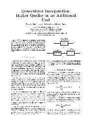
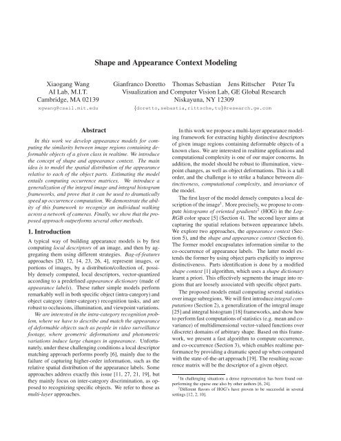
Shape and Appearance Context ModelingXiaogang WangAI Lab, M.I.T.Cambridge, MA 02139xgwang@csail.mit.eduGianfranco Doretto Thomas Sebastian Jens Rittscher Peter TuVisualization and Computer Vision Lab, GE Global ResearchNiskayuna, NY 12309{doretto,sebastia,rittsche,tu}@research.ge.comAbstractIn this work we develop appearance models for computingthe similarity between image regions containing deformableobjects of a given class in realtime. We introducethe concept of shape and appearance context. The mainidea is to model the spatial distribution of the appearancerelative to each of the object parts. Estimating the modelentails computing occurrence matrices. We introduce ageneralization of the integral image and integral histogramframeworks, and prove that it can be used to dramaticallyspeed up occurrence computation. We demonstrate the abilityof this framework to recognize an individual walkingacross a network of cameras. Finally, we show that the proposedapproach outperforms several other methods.1. IntroductionA typical way of building appearance models is by firstcomputing local descriptors of an image, and then by aggregatingthem using different strategies. Bag-of-featuresapproaches [20, 12, 14, 23, 26, 4], represent images, orportions of images, by a distribution/collection of, possiblydensely computed, local descriptors, vector-quantizedaccording to a predefined appearance dictionary (made ofappearance labels). These rather simple models performremarkably well in both specific object (intra-category) andobject category (inter-category) recognition tasks, and arerobust to occlusions, illumination, and viewpoint variations.We are interested in the intra-category recognition problem,where we have to describe and match the appearanceof deformable objects such as people in video surveillancefootage, where geometric deformations and photometricvariations induce large changes in appearance. Unfortunately,under these challenging conditions a local descriptormatching approach performs poorly [6], mainly due to thefailure of capturing higher-order information, such as therelative spatial distribution of the appearance labels. Someapproaches address exactly this issue [11, 27, 21, 19], butthey mainly focus on inter-category discrimination, as opposedto recognizing specific objects. We refer to those asmulti-layer approaches.In this work we propose a multi-layer appearance modelingframework for extracting highly distinctive descriptorsof given image regions containing deformable objects of aknown class. We are interested in realtime applications andcomputational complexity is one of our major concerns. Inaddition, the model should be robust to illumination, viewpointchanges, as well as object deformations. This is a tallorder, and the challenge is to strike a balance between distinctiveness,computational complexity, and invariance ofthe model.The first layer of the model densely computes a local descriptionof the image 1 . More precisely, we propose to computehistograms of oriented gradients 2 (HOG) in the Log-RGB color space [5] (Section 4). The second layer aims atcapturing the spatial relations between appearance labels.We explore two approaches, the appearance context (Section5), and the shape and appearance context (Section 6).The former model encapsulates information similar to theco-occurrence of appearance labels. The latter model extendsthe former by using object parts explicitly to improvedistinctiveness. Parts identification is done by a modifiedshape context [1] algorithm, which uses a shape dictionarylearnt a priori. This effectively segments the image into regionsthat are loosely associated with specific object parts.The proposed models entail computing several statisticsover image subregions. We will first introduce integral computations(Section 2), a generalization of the integral image[25] and integral histogram [18] frameworks, and show howto perform fast computations of statistics (e.g. mean and covariance)of multidimensional vector-valued functions over(discrete) domains of arbitrary shape. Based on this framework,we present a fast algorithm to compute occurrence,and co-occurrence (Section 3), which enables realtime performanceby providing a dramatic speed up when comparedwith the state-of-the-art approach [19]. The resulting occurrencematrix will be the descriptor of a given object.1 In challenging situations a dense representation has been found outperformingthe sparse one also by other authors [6, 24].2 Different flavors of HOG’s have proven to be successful in severalsettings [12, 2, 10].

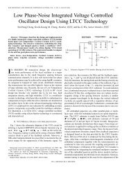
We apply our appearance models to the challengingappearance-based person reidentification 3 problem [6],which is the ability to recognize an individual across a networkof cameras based on appearance cues. We show thatthis framework can perform recognition of people appearingfrom three different viewpoints using a k-nearest neighborapproach, and achieve a significant performance increaseover the state-of-the-art approach [6].Related prior art. In [6] the authors consider a sparselocal descriptor matching approach, and a dense approachwhere body parts are automatically extracted and compared.The dense approach outperforms the sparse one. In [9]the inter-camera brightness transfer functions is learnt toperform people track-linking across multiple cameras. Althoughit would be beneficial, our work does not use thisinformation. Related work also includes vehicle reidentification[7], tracking [28], and category recognition [17, 13].In [19] the authors use the local descriptors of [26],learnt to maximize intra-category invariance, and add anotherlayer that captures the co-occurrence between appearancelabels. They show an improved inter-category discriminationover [26]. Note that our appearance modelsare meant to maximize intra-category discrimination ratherthan invariance.2. Integral computationsIn this section we introduce the unified framework of the integralcomputations, show how it specializes to the integralimage [25], and integral histogram [18], show his power incomputing statistics over rectangular domains, and extendits applicability to general, non-simply connected rectangulardomains.Given a function f(x) : R k → R m , and a rectangulardomain D = [u 1 , v 1 ] × · · · × [u k , v k ] ⊂ R k , if there existsan antiderivative 4 F(x) : R k → R m , of f(x), then∫f(x) dx = ∑(−1) νT1 F(ν 1 u 1 +¯ν 1 v 1 ,· · ·, ν k u k +¯ν k v k ) ,Dν∈B k (1)where ν = (ν 1 , · · · , ν k ) T , ν T 1 = ν 1 + · · · + ν k , ¯ν i =1 − ν i , and B = {0, 1}. If k = 1, then ∫ D f(x)dx =F(v 1 ) −F(u 1 ), which is the Fundamental Theorem of Calculus.If k = 2, then ∫ D f(x)dx = F(v 1, v 2 )−F(v 1 , u 2 )−F(u 1 , v 2 ) + F(u 1 , u 2 ), and so on.Equation (1) defines a class of operations that we callintegral computations. They are very attractive for at leastthree reasons. First, in the discrete domain one specificationof F(x) can always be found, e.g. 5 F(x) = ∑ u≤x f(u).Second, F(x) can be computed from a single pass inspec-3 If we were to apply the model to the people track-linking problem, itwould be more appropriate to talk about person reacquisition.4 If the Fubini’s theorem for indefinite integrals holds, then F(x) exists.5 Here u ≤ x is intended as u 1 ≤ x 1 , · · · , u k ≤ x k .u2,1u2,2u 2,3u2,4u2,5x 2u u u u u1,1 1,2 1,3 1,4 1,5+R R−R+R1 2 3 4RR5 6−R 7RR+R−R8 9 10 11− +RR R12 13 14+Figure 1. Generalized rectangular domain and corner types.Left: Example of a generalized rectangular domain D, partitionedinto simple rectangular domains {R i}. Right: Function α D(x).It assumes values different then zero only if x is a corner of D.The specific value depends on the type of corner. For the planarcase there are only 10 types of corner, depicted here along with thecorresponding values of α D.tion 6 of f(x), i.e. with computational cost O(N k ), whereN k represents the dimension of the discrete domain wheref(x) is defined. Finally, we will see that Equation (1) enablesthe computation of statistics over the rectangular domainD in constant time O(1), regardless of the size of D.Specific cases. If k = 2 and m = 1, and f(x) = . I(x),a grayscale image, then F(x) in Computer Vision is nowreferred to as the integral image of I(x) [25]. If f(x) =.e ◦ q ◦ I(x), where q : R → A is a quantization (labeling)function, with quantization levels A = {a 1 , · · · , a m }, ande : A → N m is such that a i ↦→ e i , where e i is the unit vectorwith only the i-th component different then 0, then F(x) isthe so called integral histogram of I(x) with respect to q[18]. In general, one has the freedom to design f(x) adlibitum, in order to take advantage of the properties of theintegral computations.Computing statistics. If x is a uniformly distributed randomvariable, and E[·|D] denotes the expectation where xis constrained to assume values in D, then one can write theexpression of simple statistics, such as the mean 7 of f(x)over DE[f(x)|D] = 1|D|or the covariance of f(x) over D∫D−x1+1−1−1+1+2f(x)dx , (2)E[(f(x) − E[f(x)|D])(f(x) − E[f(x)|D]) T |D] =∫1g(x)dx − 1 ∫|D||D|∫D2 f(x)dx f(x) T dx , (3)DDwhere g(x) : R k → R m×m is such that x ↦→ f(x)f(x) T .Similarly, higher-order moments can be written in this manner.What those expressions share is the fact that the integraloperation can be substituted with the result of Equation (1).Therefore, given F(x), their computation cost is O(1), independentfrom the size of D.6 The single pass inspection of f(x) is the k-dimensional extension ofthe 2-dimensional version described in [25, 18].7 The operation | · | applied to a domain or a set indicates the area or thecardinality, respectively.−1+1+1−1−2

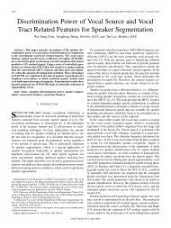
The expressions (2) and (3) assume very different meaningsaccording to the choice of f(x). For instance, for theintegral image they represent mean and covariance of thepixel intensities over the region D. On the other hand, forthe integral histogram, (2) is the histogram of the pixels ofthe region D, according to the quantization q. Recently,[22] used (3) as a region descriptor to perform object detectionand texture classification, where f(x) was the outputof a bank of filters applied to the input image I(x).Domain generalization. To the best of our knowledge theintegral computations have been used only when the regionD is rectangular. On the other hand, Equation (1) can begeneralized to domains defined as follows (see Figure 1).Definition 1. D ⊂ R k is a generalized rectangular domainif his boundary ∂D is made of a collection of portions ofa finite number of hyperplanes perpendicular to one of theaxes of R k .If ∇ ·D indicates the set of corners of a generalized rectangulardomain D, then the following result holds.Theorem 1. ∫f(x)dx = ∑α D (x)F(x) , (4)D x∈∇·Dwhere α D : R k → Z, is a map that depends on k. For k = 2it is such that α D (x) ∈ {0, ±1, ±2}, according to which ofthe 10 types of corners depicted in Figure 1, x belongs to.Theorem 1 (proved in the Appendix), says that if D is ageneralized rectangular domain, one can still compute theintegral of f(x) over D in constant time O(1). This is doneby summing up the values of F(x), computed at the cornersx ∈ ∇ ·D, and multiplied by α D (x), which depends on thetype of the corner. For the planar case the types of cornersare depicted in Figure 1. Therefore, given any discrete domainD, by simply inspecting the corners to evaluate α D ,one can compute statistics over D in constant time O(1).This simple and yet powerful result enables designing fast,more flexible and sophisticated region based features, likethe one of the following Section.3. Occurrence computationsIn this section we define the concept of occurrence, proposea new algorithm based on Theorem 1 to compute it,analyze the computational complexity of the algorithm, andcompare it to the state-of-the-art approach.Let S : Λ → S, and A : Λ → A be two functions definedon a discrete domain Λ of dimensions M ×N, and assumingvalues in the label sets S = {s 1 , · · · , s n } and A ={a 1 , · · · , a m } respectively. Also, let P = {p 1 , · · · , p l } be apartition such that ⋃ i p i represents the plane, and p i ∩p j =∅, if i ≠ j (see Figure 2 for an example). Given p ∈ P, anda point on the plane x, we define p(x) . = {x + y|y ∈ p},and we indicate with h(a, p(x)) . = P[A(y) = a|y ∈ p(x)]the probability distribution 8 of the labels of A over the re-8 P[·] indicates a probability measure.p3p p 1 2p6p p 4 5x1p7x2Ss 1.. ... . ..xs3... .s 5..s2s4Ap( x)4a2a1a3ss 3ΘΘ(a,s ,p )3 4Figure 2. Partition and occurrence definition. From left to right.Example of a generic partition P. Example of a function S, andof a function A. Representation of Θ. If h(a, p 4(x)) is thenormalized count of the labels of A in p 4(x) (the partition elementp 4 translated at x), then by averaging h(a, p 4(x)) over allx ∈ {y|S(y) = s 3} . = D s3 , we obtain Θ(a, s 3, p 4) (red line).The dots over S highlight the corner points ∇ · D s3 .gion p(x). In other words, for a given A, if we randomlyselect a point y ∈ p(x), the probability that the label atthat point will be a is given by h(a, p(x)). If we now set.D s = {x|S(x) = s}, s ∈ S, we define the occurrencefunction as follows (see Figure 2).Definition 2. The occurrence function Θ : A × S × P →R + , is such that the point (a, s, p) maps toΘ(a, s, p) = E[h(a, p(x))|D s ] . (5)The meaning of the occurrence function is the following:Given S and A, if we randomly select a point x ∈ D s , theprobability distribution of the labels A over the region p(x)of A is given by Θ(·, s, p). One special case is when S = A,and S(x) = A(x), and Θ is typically referred to as cooccurrence.When Θ is intended as a collection of valuescorresponding to all the points of the domain A × S × P,we refer to it as the occurrence, or co-occurrence matrix.3.1. Fast occurrence computationIn this section we present a novel result that allows a fastcomputation of the occurrence function. The derivation isbased on the fact that the occurrence is computed over a discretedomain Λ, where every possible sub-domain is a (discrete)generalized rectangular domain, and all the results ofSection 2 can be applied.Theorem 2. The occurrence function (5) is equal toΘ(a, s, p) = |D s | −1 |p| −1 ∑where G(·,x) =x∈∇·D s,y∈∇·p∫ x−∞∫ u−∞α Ds (x)α p (y)G(a,x+y) ,p 4ap(6)e ◦ A(v)dv du , (7)and 9 e : A → N m is such that the inner integral is theintegral histogram of A.Theorem 2 (proved in the Appendix) leads to the Algorithm1. We point out that even though the occurrence hasbeen introduced for S and A defined on a two-dimensional9 Note that a ∈ A is intended to index one of the elements of the m-dimensional vector G(·,x).

Algorithm 1: Fast occurrence computation12345Data: Functions A and SResult: Occurrence matrix ΘbeginUse (7) to compute G from a single pass inspection of A// Compute |D s| α Ds and ∇ · D sforeach x ∈ Λ do|D S(x) | ←− |D S(x) | + 1ifIsCorner (x) thenSet α DS(x) (x)6S 7 ∇ · D S(x) ←− ∇ · D S(x) {x}// Use (6) to compute Θ// |p| α p and ∇ · p known a priori8 foreach s ∈ S do9 foreach p ∈ P do10foreach x ∈ ∇ · D s do11foreach y ∈ ∇ · p do12Θ(·, s, p) ←− Θ(·, s, p)+13α Ds (x)α p(y)G(·,x + y)1415 return Θ16 endΘ(·, s, p) ←− |D s| −1 |p| −1 Θ(·, s, p)domain, the definition can be generalized to any dimension,and Theorem 2 still holds.Complexity analysis. Given S and A, the na¨ive approachto compute Θ costs O(N 4 ) in time (we assume M ∼ N),which is too much for real-time applications, even if N isnot very large. In [8] a dynamic programming approachreduces the cost to O(N 3 ). In [19] a particular partition Pwhere every p ∈ P is a square ring defined by |∇ · p| = 8corners enables a computation cost 10 of O(N 2 l|∇ · p|) =O(N 2 .C P ), where C P = l|∇·p| represents the total numberof corners of P.We now calculate the computational cost of Algorithm 1.Line 2 can be evaluated by a single pass inspection of A, andhas the same computational cost of an integral histogram,i.e. O(N 2 ). Line 3-7 is another single pass inspection of Swith cost O(N 2 ). Line 12 costs O(1). Line 11 is an average.multiplying factor of C P /l, where C P =∑i |∇ · p i|. Line.∑10 is an average multiplying factor of C S /n, where C S =i |∇ · D s i|. Line 8 and 9 are multiplying factors of nand l respectively. Therefore, the cost of 8-13 is O(C S C P ).Finally, the total cost of Algorithm 1 is O(N 2 + C S C P ).In practice we have C s C P ∼ N 2 . Therefore, Algorithm 1has an effective cost of O(N 2 ), which is C P (the number ofcorner points of the partition P) times faster then the stateof-the-art[19]. It is interesting to note that Algorithm 1 isonly marginally sensitive to the choice of the partition P,which, as opposed to [19], here is allowed to be arbitrary.10 In [19] |∇ · p| is part of the hidden constants. Here we make thedependency explicit to better compare their approach with ours.4. Bag-of-features modelingIn this section, as well as in Sections 5 and 6, we are interestedin designing a highly distinctive descriptor for animage I, belonging to I, the space of all the images definedon a discrete domain Λ of dimensions M × N pixels.To this end we process the image by applying an operatorΦ : I × Λ → R r , such that (I,x) is mapped to a local descriptorϕ(x) . = Φ(I,x). The operator Φ could be a bankof linear filters, as well as any other non-linear operation.Once ϕ is available, the descriptor is computed in twosteps. The first one performs a vector quantization of ϕ,according to a quantization function q : R r → A, withquantization levels A = {a 1 , · · · , a m }. This produces theappearance labeled image A(x) . = q ◦ ϕ(x) (see Figure 3for an example). We refer to A as the appearance dictionary,made of appearance labels learnt a priori. The secondstep computes the histogram of the labels h : A → [0, 1],such that the label a maps toh(a) . = P[A(x) = a] . (8)The image descriptor is defined to be the histogram h.HOG Log-RGB operator. In Section 7 we experimentwith several operators Φ, such as different color spaces andfilter banks, and test their matching performance with thedescriptor (8). The best performer operates in the RGBcolor space, and is such that ϕ(x) = . (HOG(∇ log(I R ),x);HOG(∇ log(I G ),x); HOG(∇ log(I B ),x)), where I R , I G ,I B , are the R, G, and B channels of I respectively. Theoperator HOG(·,x) computes the l bins histogram of orientedgradients of the argument, on a region of w × w pixelsaround x. The gradient of the Log-RGB space has aneffect similar to the homomorphic filtering, and makes thedescriptor robust to illumination changes.5. Appearance context modelingThe main drawback of the bag-of-features model is that imagesof different objects that share the same appearance labeldistribution h(a), share also the same descriptor, annihilatingthe distinctiveness that we are seeking. This is due tothe fact that (8) does not incorporate any description of howthe object appearance is distributed in space. On the otherhand, this information could be captured by computing thespatial co-occurrence between appearance labels.Appearance context. More precisely, the co-occurrencematrix Θ, computed on the appearance labeled image A(x)with the plane partition P depicted in Figure 4, will be referredto as the appearance context descriptor of I, whichis an m × m × l matrix.Appearance context vs. bag-of-features. Note that theinformation carried by the descriptor (8) is included in theappearance context descriptor. In fact, by using (6) one canshow that Θ reduces to (8), in particular, for every b ∈ Awe have h(a) = 1/|Λ| ∑ p∈P|p|Θ(a, b, p).

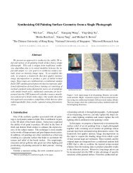
Figure 3. Data set and shape and appearance labeled images.From left to right. Two samples from the data set of 143 differentindividuals, recorded from 3 different viewpoints, with correspondingshape labeled image S, and appearance labeled imageA. Note that the decomposition into parts performed by S triesto compensate the misalignment induced by pose and viewpointchanges, as well as person bounding box imprecisions.Plane partition. P is made of p 1 , · · · , p l , L-shaped regions.Every quadrant is covered by l/4 regions. EveryL-shape is 4N/l and 4M/l thick along the x 1 and x 2 directions,respectively. Therefore, the set {p i } can be partitionedinto groups of 4 elements forming l/4 correspondingconcentric square rings.Invariance. It is known that the co-occurrence matrix istranslation invariant, rotation invariant if the {p i } are concentriccircular rings, and shows robustness to affine andpose changes [8, 19]. It is not invariant with respect to thesize of I. In order to have this property, before computingthe appearance context we will normalize the size of I. Themorphology of the partition P makes the appearance contextnon-rotation invariant. In our application this is a desiredproperty as it increases distinctiveness. In fact, lack ofrotation invariance allows us to distinguish between a personwearing a white T-shirt and black pants vs. a personwearing a black T-shirt and white pants.6. Shape and appearance context modelingLet’s now consider a toy example to highlight an importantweakness of the appearance context descriptor, and examinethe appearance labeled image of a person depicted inFigure 4 (right). We indicate with D f and D h the face andhand regions respectively, and notice that these are the onlyregions that have been assigned the label a 1 ∈ A. Using thenotation introduced in Section 3, we also have D a1 = D f ∪D h . The region of the torso, arm, and hair has been assignedthe label a 2 ∈ A. For a 1 and a 2 the appearance contextcan be rewritten as Θ(a 2 , a 1 , p) = D fD a1E[h(a 2 , p)|D f ] +D h.D a1E[h(a 2 , p)|D h ] = h f (p) + h h (p). Note that h f (p),(h h (p)), is the occurrence of a 2 at a given distance and orientationfrom D f , (D h ), defined by p. Figure 4 sketchesh f (p), h h (p), and their sum. h f (p) highlights that a 2 ismostly present in the blue and yellow quadrants of the partitionP. h h (p) highlights that a 2 is mostly present in thered and green quadrants of the partition P. h f (p) + h h (p)shows that a 2 is uniformly distributed over all the quadrants.We point out that averaging h f and h h has caused a lossof information, and therefore descriptive power. From ana 1 =a 2 =+x 1γ 2x 2 γ 1Figure 4. L-shaped partition and appearance context averagingeffect. From left to right. Sketch of the L-shaped plane partitionused in Section 5 (γ 1 = 4N/l, γ 2 = 4M/l), and 6 (γ 1 = 4Nd/t,γ 2 = 4Md/t). Illustration of the averaging effect when appearancecontext descriptors are pooled from the entire object region.information theoretic point of view, two unimodal distributionshave been merged to obtain an almost uniform distribution,with a significant increase of entropy. To preventsuch a situation, this toy example suggests that if we couldidentify the parts of a given object, it would be more descriptiveto capture the spatial occurrence of the appearancelabels with respect to each of the parts rather then toeach of the appearance labels.Shape and appearance context. Given I containing anobject of a given class, let A be its appearance labeled image,and let S (defined over Λ) be its shape labeled image,where pixel labels are meant to identify regions of I occupiedby specific parts of the object (see Figure 3 for examples).We define the shape and appearance context descriptorof I, the occurrence matrix Θ, computed over S and A,which is an m × n × l matrix. Similarly to the appearancecontext descriptor, the information carried by the descriptor(8) is included in the shape and appearance context descriptor.Shape labeled image. We propose to compute the shapelabeled image with a procedure that is inspired by the ideaof shape context [1, 16]. Given the image I ∈ I, we processit according to an operator Ω : I × Λ → R d , suchthat I is mapped to ω(x) = . Ω(I,x). In Section 7 we considerdifferent operators Ω. A fast and reliable choice issuch that ω(x) = HOG(∇I L ,x), where I L is the L channelof the Lab color space of I. From ω, at every pixelwe compute a form of shape context descriptor ψ, definedas ψ(x) = . (E[ω|p 1 (x)]; · · · ; E[ω|p t/d (x)]) ∈ R t . Here{p 1 , · · · , p t/d } indicates a plane partition of the same kindused for the appearance context descriptor, but with t/dL-shaped regions rather then l (see Figure 4). Once ψ isavailable, we vector quantize it according to a quantization(labeling) function q : R t → S, with quantization levelsdefined by a shape dictionary S = {s 1 , · · · , s n }, made ofshape labels learnt a priori. This produces the shape labeledimage S(x) = . q ◦ ψ(x).Neighboring pixels have similar shape context descriptors.Therefore, the quantization process produces a“piecewise-like” segmentation of the image into regionsD si = {x|S(x) = s i }, which are meant to always identifythe same region/part of the object of interest (see Figure 3).=h fh h

Matching Rate0.90.80.70.60.5Lab 5−5−5 pls0.4Lab 5−5−5 mulRGB 4−4−4 pls0.3RGB 4−4−4 mul0.2HSV 16−3−3 plsHSV 16−3−3 mul0.10 5 10 15 20K−nearest neighborMatching Rate0.80.70.60.50.40.30.2m=30m=40m=50m=60m=70m=1005 10 15 20K−nearest neighborFigure 5. Bag-of-features: Color spaces and linear filters.Matching comparison using different color spaces and quantizationschemes (left). Matching comparison of a linear filter bankagainst appearance dictionary size (right).As a welcome side effect, the occurrence computation takesgreat advantage of this segmentation, as C S ends up beingvery small.Invariance. The shape and appearance context enjoys thesame invariance properties of the appearance context. However,it should be noted that translation invariance is lost ifthe same parts of an object are labeled differently in differentimages, e.g. an arm labeled as a leg. This meansthat using a fixed mask to identify object parts under poseand viewpoint changes, as well as object bounding box imprecisions,significantly decreases the performance of thedescriptor. The decomposition into parts with the shapelabeled image tries to compensate exactly those variations(see Figure 3).7. ExperimentsData set. The data set is composed by the one in [6], containing44 different individuals recorded from three differentnon-overlapping camera views (see Figure 3), to whichwe added new images of 99 individuals, recorded from threevery similar viewpoints. Every person in each view is representedby two to four images, of about 80 × 170 pixelsin size. In a video-surveillance system such images wouldbe cropped out of the full frames by a person detector, ortracker module.Matching. As in [6], for every pair person/camera view,we compute the k-nearest people in the other views. Sinceevery pair is represented by a number of images, the distancebetween two pairs is the minimum distance betweentwo images (that do not belong to the same pair), measuredaccording to a given distance between descriptors.Identification results are reported in terms of cumulativematch characteristic (CMC) curves [15], which tell the rateat which the correct match is within the k-nearest neighbors,with k that varies from 1 to 20.Training and testing. The appearance and shape dictionariesare learnt using simple k-means clustering after computingϕ and ψ on the training set, respectively. For training,we used the images of 30% of the individuals randomlyselected. The rest of the data set was used for testing.Distances. Appearance labels are learned and assigned usingL 1 norm. Shape labels are learned and assigned usingMatching RateMatching Rate10.90.80.70.60.50.410.90.80.70.60.50.40.38 bins10 bins12 bins14 bins16 bins18 bins5 10 15 20K−nearest neighborPatch size = 5Patch size = 7Patch size = 9Patch size = 11Patch size = 13Patch size = 155 10 15 20K−nearest neighborMatching RateMatching Rate10.90.80.70.60.50.410.90.80.70.60.50.4σ = 0.0σ = 0.5σ = 1.0σ = 2.0σ = 3.05 10 15 20K−nearest neigborm=30m=40m=50m=60m=705 10 15 20K−neares neighborFigure 6. Bag-of-features: HOG Log-RGB. Matching comparisonby varying one of the operator parameters at a time, suchas the quantizing orientations l (top-left), the image smoothing σ(top-right), the patch size w (bottom-left), and the appearance dictionarydimensionality m (bottom-right).the χ 2 distance 11 . Descriptor matching using (8) is donewith the intersection distance (used also in [6]). Descriptormatching using appearance, and shape and appearancecontext is done with L 1 norm.Bag-of-features: Color spaces and linear filters. Figure5 (left) shows results where Φ is a color transformationand quantization. We tried the Lab, RGB, and HSVcolor spaces, quantized along the three axes according tothe number of bins reported in the figure. The suffixes“pls” and “mul” indicate whether channel quantization isperformed independently, or jointly. The Lab and the RGBcolor spaces seem to perform better. In Figure 5 (right), Φis the linear filter (LF) bank used in [26]. It shows that linearfiltering improves versus simple color quantization, andthat there is an optimal dimensionality for A, say aroundm = 60.Bag-of-features: HOG Log-RGB. Figure 6 summarizesour search for optimal settings for computing HOG’s. Weoptimize four parameters (one at a time): the number ofquantizing orientations l, the prior Gaussian smoothing ofthe image σ, the patch size w, and the appearance dictionarydimensionality m. We found a good operating point 12 withl = 16, σ = 0, w = 11, and m = 60.Shape descriptors. For computing ω, the HOG uses d = 8quantizing orientations, a patch size w = 11, and a shapedictionary of dimension n = 18. Note that there might beother ways to design the operator 13 Ω.11 Note that ψ is a concatenation of histograms.12 We tested the HOG with other color spaces. The L channel and theLog-RGB color space are the best options. They double the performancewith respect to the linear filter bank (CMC curves included in [3]).13 We experimented a Canny edge detector, where ψ does an edge pixelscount on the partition regions. This approach compares well with the HOG,

Matching Rate10.90.80.70.60.5HOG in Log−RGBHOG in RGBHOG in color−ratio spaceLF + HOG in L channelLF0.40 5 10 15 20K−nearest neighborMatching Rate10.90.80.70.60.50.40.30.20.1RGB histogramHSV histogramLab histogramLF histogramHOG Log−RGB histogramCorrelaton histogramCorrelaton +LF histogramShape and appearance c.Appearance contextModel Fitting00 2 4 6 8 10 12 14 16 18 20K−nearest neighborFigure 7. Shape and appearance context. Left: Matching comparisonbetween several approaches for computing appearancelabels. Approaches using HOG outperform the ones that donot. Right: Matching comparison summary of several appearancemodels. The shape and appearance context outperforms all others,including the state-of-the-art model fitting [6]. Approaches thatcapture spatial relationships outperform those that do not.Shape and appearance context: Appearance comparison.Figure 7 (left) shows the results corresponding todifferent choices of Φ. We tested the HOG in three differentcolor spaces. We also tested the linear filter bank (LF)used in [26], and a combination of the LF and the HOGof the L channel of the Lab color space. It is noticeablehow the configurations that include the HOG significantlyoutperform the LF bank. The HOG in the Log-RGB colorspace is the best performer.Comparison summary. Figure 7 (right) compares thematching performance of several approaches. Besides appearanceand shape and appearance context, we have includedsimple bag-of-features approaches where Φ is acolor transformation (to spaces such as RGB, HSV, Lab),but also more sophisticated ones, where Φ is a LF bank[26], or the HOG in the Log-RGB space. Results usingthe histogram of correlatons, 14 and his concatenation withthe histogram (8), where Φ is the LF bank [19] are also included.The results indicate that the shape and appearance contextis the best performing algorithm. Further, approachesthat capture the spatial relationships among appearance labelssignificantly outperform the approaches that do not,such as bag-of-features. Finally, the comparison with themodel fitting algorithm [6], shows that the matching rate ofthe first neighbor is 59%, whereas for the shape and appearancecontext it is 82%, which is a significant improvement(see Figure 7).8. ConclusionsWe propose the shape and appearance context, an appearancemodel that captures the spatial relationshipsamong appearance labels. This outperforms other methods,especially in very challenging situations, such as thewith a slight advantage to the latter (CMC curves included in [3]).14 We have used our own implementation of the algorithm [19]. Learningwas done with k-means only. We warn the reader that their approach wasoriginally designed to solve the inter-category recognition problem, andhere we have tested it outside his natural domain.appearance-based person reidentification problem. In thisscenario, our extensive testing to design several operatorshas led to a method that achieves a matching rate of 82% ona large data set.The new algorithm to compute occurrence, which cutsthe computational complexity down to O(N 2 ), enables thecomputation of the shape and appearance context in realtime,15 which is not possible using existing methods. Thecomputation of the occurrence is based on the proposed integralcomputations framework, which generalizes the ideasof integral image and integral histogram to multidimensionalvector-valued functions, and allows computing statisticsover discrete domains of arbitrary shape.The appearance variation of our testing data set showsthat our approach is robust to a great deal of viewpoint, illumination,and pose changes, not to mention backgroundcontamination. Future investigation will include methodsto remove this contamination, and testing the approach inother scenarios, e.g. multiple hypothesis tracking.AppendixIn this Appendix we first introduce some notation and thengive the proofs of Theorem1, and 2. The variable ν canbe interpreted as partitioning R k into his 2 k open orthants.O ν = {x ∈ R k |x i > 0 if ν i = 1, or x i < 0 if ν i = 0, i =1, · · · , k}. We introduce the notation O ν (x) = . {x+y|y ∈O ν }. We also introduce a function β x (ν) : B k → B, suchthat: i) β x (ν) = 1 if x is an adherent point 16 for the openset D ∩ O ν (x); ii) β x (ν) = 0 otherwise. It is trivial toprove that: I) x ∈ D \ ∂D ⇐⇒ β x (ν) = 1 ∀ν; II) x ∈\ D⇐⇒ β x (ν) = 0 ∀ν. Finally, if ν j represents j out of thek components of ν, and if ν k−j represents the remainingk − j components, then we define edges and corners of theboundary ∂D as follows: A point x ∈ ∂D lays on an edgeif there exist j components of ν, with 1 ≤ j ≤ k − 1, suchthat β x (ν) does not depend on ν k−j , i.e. β x (ν) = β x (ν j ),∀ν. If x does not lay on an edge, it is a corner. We indicatethe set of corners with ∇ · D.Proof of Theorem 1. Let {u i,1 , u i,2 , · · · |u i,j ∈ R, u i,j

and α D (x) = . ∑ ν (−1)νT1 β x (ν). Now we recall that ifx ∈ D \ ∂D, then β x (ν) = 1, and this implies α D (x) = 0.On the other hand, if x is on an edge, then we can writeα D (x) = ∑ ν j(−1) νT j 1 β x (ν j ) ∑ ν k−j(−1) νT k−j 1 = 0,and Equation (4) is valid. When x is a corner describedby β x , one should proceed with a direct computation ofα D (x). For k = 2, α D (x) is different then zero only forthe 10 cases depicted in Figure 1, in which it assumes thevalues indicated.□Proof of Theorem 2. According to (5), Θ can be computedby using Equation (2), and subsequently applyingTheorem 1, givingΘ(a, s, p) = |D s | −1where H(a, p(x)) =∑x∈∇·D sα Ds (x)H(a, p(x)) , (9)∫ x−∞h(a, p(u))du . (10)Now we note that h(a, p(u)) can be computed throughthe integral histogram of A, F(a,z) = ∫ z−∞ e ◦ A(v)dv,and by applying Theorem 1, resulting in h(a, p(u)) =|p(u)| −1∑ z∈∇·p(u) α p(u)(z)F(a,z). This equation, combinedwith Equations (10) gives∫ xH(a, p(x)) = |p(u)| ∑ −1 α p(u) (z)F(a,z)du . (11)−∞z∈∇·p(u)From the definition of p(u), it follows that |p(u)| = |p|,and ∇ · p(u) = {u + y|y ∈ ∇ · p}, and also thatα p(u) (u +y) = α p (y). Therefore, after the change of variablez = u + y, in Equation (11) it is possible to switchthe order between the integral and the summation, yieldingH(a, p(x)) = |p| −1∑ y∈∇·p α p(y) ∫ xF(a,u + y)du.−∞Substituting this expression in (9), and taking into accountthe expression of F(a,z), proves Equations (6) and (7). □AcknowledgementsThis report was prepared by GE GRC as an account of work sponsored byLockheed Martin Corporation. Information contained in this report constitutestechnical information which is the property of Lockheed MartinCorporation. Neither GE nor Lockheed Martin Corporation, nor any personacting on behalf of either; a. Makes any warranty or representation,expressed or implied, with respect to the use of any information containedin this report, or that the use of any information, apparatus, method, or processdisclosed in this report may not infringe privately owned rights; or b.Assume any liabilities with respect to the use of, or for damages resultingfrom the use of, any information, apparatus, method or process disclosedin this report.References[1] S. Belongie, J. Malik, and J. Puzicha. Shape matching and objectrecognition using shape contexts. IEEE TPAMI, 24:509–522, 2002.[2] N. Dalai and B. Triggs. Histograms of oriented gradients for humandetection. In CVPR, volume 1, pages 886–893, June 20–25, 2005.[3] G. Doretto, X. Wang, T. B. Sebastian, J. Rittscher, and P. Tu. Shapeand appearance context modeling: A fast framework for matching theappearance of people. Technical Report 2007GRC594, GE GlobalResearch, Niskayuna, NY, USA, 2007.[4] L. Fei-Fei and P. Perona. A Bayesian hierarchical model for learningnatural scene categories. In CVPR, volume 2, pages 524–531, June20–25, 2005.[5] B. V. Funt and G. D. Finlayson. Color constant color indexing. IEEETPAMI, 17:522–529, 1995.[6] N. Gheissari, T. B. Sebastian, P. H. Tu, J. Rittscher, and R. Hartley.Person reidentification using spatiotemporal appearance. In CVPR,volume 2, pages 1528–1535, 2006.[7] Y. Guo, S. Hsu, Y. Shan, H. Sawhney, and R. Kumar. Vehicle fingerprintingfor reacquisition & tracking in videos. In CVPR, volume 2,pages 761–768, June 20–25, 2005.[8] J. Huang, S. R. Kumar, M. Mitra, W.-J. Zhu, and R. Zabih. Imageindexing using color correlograms. In CVPR, pages 762–768, SanJuan, June 17–19, 1997.[9] O. Javed, K. Shafique, and M. Shah. Appearance modeling for trackingin multiple non-overlapping cameras. In CVPR, volume 2, pages26–33, June 20–25, 2005.[10] S. Kumar and M. Hebert. Discriminative random fields. IJCV,68:179–201, 2006.[11] S. Lazebnik, C. Schmid, and J. Ponce. Affine-invariant local descriptorsand neighborhood statistics for texture recognition. In ICCV,pages 649–655, 2003.[12] D. Lowe. Distinctive image features from scale-invariant key points.IJCV, 60:91–110, 2004.[13] X. Ma and W. E. L. Grimson. Edge-based rich representation forvehicle classification. In CVPR, volume 2, pages 1185–1192, Oct.17–21, 2005.[14] K. Mikolajczyk and C. Schmid. A performance evaluation of localdescriptors. IEEE TPAMI, 27:1615–1630, 2005.[15] H. Moon and P. J. Phillips. Computational and performance aspectsof PCA-based face-recognition algorithms. Perception, 30(3):3003–321, 2001.[16] G. Mori and J. Malik. Recovering 3d human body configurationsusing shape contexts. IEEE TPAMI, 28(7):1052–1062, July 2006.[17] O. C. Ozcanli, A. Tamrakar, B. B. Kimia, and J. L. Mundy. Augmentingshape with appearance in vehicle category recognition. InCVPR, volume 1, pages 935–942, New York, NY, USA, 2006.[18] F. Porikli. Integral histogram: a fast way to extract histograms incartesian spaces. In CVPR, volume 1, pages 829–836, June 20–25,2005.[19] S. Savarese, J. Winn, and A. Criminisi. Discriminative object classmodels of appearance and shape by correlatons. In CVPR, volume 2,pages 2033–2040, 2006.[20] B. Schiele and J. L. Crowley. Recognition without correspondenceusing multidimensional receptive field histograms. IJCV, 36(1):31–50, 2000.[21] J. Shotton, J. Winn, C. Rother, and A. Criminisi. Textonboost: Jointappearance, shape and context modeling for multi-class object recognitionand segmentation. In ECCV, pages 1–15, 2006.[22] O. Tuzel, F. Porikli, and P. Meer. Region covariance: A fast descriptorfor detection and classification. In ECCV, pages 589–600, 2006.[23] M. Varma and A. Zisserman. A statistical approach to texture classificationfrom single images. IJCV, 62:61–81, 2005.[24] A. Vedaldi and S. Soatto. Local features, all grown up. In CVPR,volume 2, pages 1753–1760, 2006.[25] P. Viola and M. J. Jones. Robust real-time face detection. IJCV,57:137–154, 2004.[26] J. Winn, A. Criminisi, and T. Minka. Object categorization bylearned universal visual dictionary. In ICCV, volume 2, pages 1800–1807, Oct. 17–21, 2005.[27] L. Wolf and S. Bileschi. A critical view of context. IJCV, 69(2):251–261, Aug. 2006.[28] Q. Zhao and H. Tao. Object tracking using color correlogram. InVS-PETS, pages 263–270, Oct. 15–16, 2005.