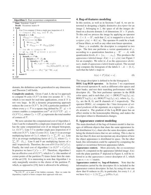
Algorithm 1: Fast occurrence computation12345Data: Functions A <strong>and</strong> SResult: Occurrence matrix ΘbeginUse (7) to compute G from a single pass inspection of A// Compute |D s| α Ds <strong>and</strong> ∇ · D sforeach x ∈ Λ do|D S(x) | ←− |D S(x) | + 1ifIsCorner (x) thenSet α DS(x) (x)6S 7 ∇ · D S(x) ←− ∇ · D S(x) {x}// Use (6) to compute Θ// |p| α p <strong>and</strong> ∇ · p known a priori8 foreach s ∈ S do9 foreach p ∈ P do10foreach x ∈ ∇ · D s do11foreach y ∈ ∇ · p do12Θ(·, s, p) ←− Θ(·, s, p)+13α Ds (x)α p(y)G(·,x + y)1415 return Θ16 endΘ(·, s, p) ←− |D s| −1 |p| −1 Θ(·, s, p)domain, the definition can be generalized to any dimension,<strong>and</strong> Theorem 2 still holds.Complexity analysis. Given S <strong>and</strong> A, the na¨ive approachto compute Θ costs O(N 4 ) in time (we assume M ∼ N),which is too much for real-time applications, even if N isnot very large. In [8] a dynamic programming approachreduces the cost to O(N 3 ). In [19] a particular partition Pwhere every p ∈ P is a square ring defined by |∇ · p| = 8corners enables a computation cost 10 of O(N 2 l|∇ · p|) =O(N 2 .C P ), where C P = l|∇·p| represents the total numberof corners of P.We now calculate the computational cost of Algorithm 1.Line 2 can be evaluated by a single pass inspection of A, <strong>and</strong>has the same computational cost of an integral histogram,i.e. O(N 2 ). Line 3-7 is another single pass inspection of Swith cost O(N 2 ). Line 12 costs O(1). Line 11 is an average.multiplying factor of C P /l, where C P =∑i |∇ · p i|. Line.∑10 is an average multiplying factor of C S /n, where C S =i |∇ · D s i|. Line 8 <strong>and</strong> 9 are multiplying factors of n<strong>and</strong> l respectively. Therefore, the cost of 8-13 is O(C S C P ).Finally, the total cost of Algorithm 1 is O(N 2 + C S C P ).In practice we have C s C P ∼ N 2 . Therefore, Algorithm 1has an effective cost of O(N 2 ), which is C P (the number ofcorner points of the partition P) times faster then the stateof-the-art[19]. It is interesting to note that Algorithm 1 isonly marginally sensitive to the choice of the partition P,which, as opposed to [19], here is allowed to be arbitrary.10 In [19] |∇ · p| is part of the hidden constants. Here we make thedependency explicit to better compare their approach with ours.4. Bag-of-features modelingIn this section, as well as in Sections 5 <strong>and</strong> 6, we are interestedin designing a highly distinctive descriptor for animage I, belonging to I, the space of all the images definedon a discrete domain Λ of dimensions M × N pixels.To this end we process the image by applying an operatorΦ : I × Λ → R r , such that (I,x) is mapped to a local descriptorϕ(x) . = Φ(I,x). The operator Φ could be a bankof linear filters, as well as any other non-linear operation.Once ϕ is available, the descriptor is computed in twosteps. The first one performs a vector quantization of ϕ,according to a quantization function q : R r → A, withquantization levels A = {a 1 , · · · , a m }. This produces theappearance labeled image A(x) . = q ◦ ϕ(x) (see Figure 3for an example). We refer to A as the appearance dictionary,made of appearance labels learnt a priori. The secondstep computes the histogram of the labels h : A → [0, 1],such that the label a maps toh(a) . = P[A(x) = a] . (8)The image descriptor is defined to be the histogram h.HOG Log-RGB operator. In Section 7 we experimentwith several operators Φ, such as different color spaces <strong>and</strong>filter banks, <strong>and</strong> test their matching performance with thedescriptor (8). The best performer operates in the RGBcolor space, <strong>and</strong> is such that ϕ(x) = . (HOG(∇ log(I R ),x);HOG(∇ log(I G ),x); HOG(∇ log(I B ),x)), where I R , I G ,I B , are the R, G, <strong>and</strong> B channels of I respectively. Theoperator HOG(·,x) computes the l bins histogram of orientedgradients of the argument, on a region of w × w pixelsaround x. The gradient of the Log-RGB space has aneffect similar to the homomorphic filtering, <strong>and</strong> makes thedescriptor robust to illumination changes.5. <strong>Appearance</strong> context modelingThe main drawback of the bag-of-features model is that imagesof different objects that share the same appearance labeldistribution h(a), share also the same descriptor, annihilatingthe distinctiveness that we are seeking. This is due tothe fact that (8) does not incorporate any description of howthe object appearance is distributed in space. On the otherh<strong>and</strong>, this information could be captured by computing thespatial co-occurrence between appearance labels.<strong>Appearance</strong> context. More precisely, the co-occurrencematrix Θ, computed on the appearance labeled image A(x)with the plane partition P depicted in Figure 4, will be referredto as the appearance context descriptor of I, whichis an m × m × l matrix.<strong>Appearance</strong> context vs. bag-of-features. Note that theinformation carried by the descriptor (8) is included in theappearance context descriptor. In fact, by using (6) one canshow that Θ reduces to (8), in particular, for every b ∈ Awe have h(a) = 1/|Λ| ∑ p∈P|p|Θ(a, b, p).
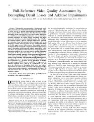
Figure 3. Data set <strong>and</strong> shape <strong>and</strong> appearance labeled images.From left to right. Two samples from the data set of 143 differentindividuals, recorded from 3 different viewpoints, with correspondingshape labeled image S, <strong>and</strong> appearance labeled imageA. Note that the decomposition into parts performed by S triesto compensate the misalignment induced by pose <strong>and</strong> viewpointchanges, as well as person bounding box imprecisions.Plane partition. P is made of p 1 , · · · , p l , L-shaped regions.Every quadrant is covered by l/4 regions. EveryL-shape is 4N/l <strong>and</strong> 4M/l thick along the x 1 <strong>and</strong> x 2 directions,respectively. Therefore, the set {p i } can be partitionedinto groups of 4 elements forming l/4 correspondingconcentric square rings.Invariance. It is known that the co-occurrence matrix istranslation invariant, rotation invariant if the {p i } are concentriccircular rings, <strong>and</strong> shows robustness to affine <strong>and</strong>pose changes [8, 19]. It is not invariant with respect to thesize of I. In order to have this property, before computingthe appearance context we will normalize the size of I. Themorphology of the partition P makes the appearance contextnon-rotation invariant. In our application this is a desiredproperty as it increases distinctiveness. In fact, lack ofrotation invariance allows us to distinguish between a personwearing a white T-shirt <strong>and</strong> black pants vs. a personwearing a black T-shirt <strong>and</strong> white pants.6. <strong>Shape</strong> <strong>and</strong> appearance context modelingLet’s now consider a toy example to highlight an importantweakness of the appearance context descriptor, <strong>and</strong> examinethe appearance labeled image of a person depicted inFigure 4 (right). We indicate with D f <strong>and</strong> D h the face <strong>and</strong>h<strong>and</strong> regions respectively, <strong>and</strong> notice that these are the onlyregions that have been assigned the label a 1 ∈ A. Using thenotation introduced in Section 3, we also have D a1 = D f ∪D h . The region of the torso, arm, <strong>and</strong> hair has been assignedthe label a 2 ∈ A. For a 1 <strong>and</strong> a 2 the appearance contextcan be rewritten as Θ(a 2 , a 1 , p) = D fD a1E[h(a 2 , p)|D f ] +D h.D a1E[h(a 2 , p)|D h ] = h f (p) + h h (p). Note that h f (p),(h h (p)), is the occurrence of a 2 at a given distance <strong>and</strong> orientationfrom D f , (D h ), defined by p. Figure 4 sketchesh f (p), h h (p), <strong>and</strong> their sum. h f (p) highlights that a 2 ismostly present in the blue <strong>and</strong> yellow quadrants of the partitionP. h h (p) highlights that a 2 is mostly present in thered <strong>and</strong> green quadrants of the partition P. h f (p) + h h (p)shows that a 2 is uniformly distributed over all the quadrants.We point out that averaging h f <strong>and</strong> h h has caused a lossof information, <strong>and</strong> therefore descriptive power. From ana 1 =a 2 =+x 1γ 2x 2 γ 1Figure 4. L-shaped partition <strong>and</strong> appearance context averagingeffect. From left to right. Sketch of the L-shaped plane partitionused in Section 5 (γ 1 = 4N/l, γ 2 = 4M/l), <strong>and</strong> 6 (γ 1 = 4Nd/t,γ 2 = 4Md/t). Illustration of the averaging effect when appearancecontext descriptors are pooled from the entire object region.information theoretic point of view, two unimodal distributionshave been merged to obtain an almost uniform distribution,with a significant increase of entropy. To preventsuch a situation, this toy example suggests that if we couldidentify the parts of a given object, it would be more descriptiveto capture the spatial occurrence of the appearancelabels with respect to each of the parts rather then toeach of the appearance labels.<strong>Shape</strong> <strong>and</strong> appearance context. Given I containing anobject of a given class, let A be its appearance labeled image,<strong>and</strong> let S (defined over Λ) be its shape labeled image,where pixel labels are meant to identify regions of I occupiedby specific parts of the object (see Figure 3 for examples).We define the shape <strong>and</strong> appearance context descriptorof I, the occurrence matrix Θ, computed over S <strong>and</strong> A,which is an m × n × l matrix. Similarly to the appearancecontext descriptor, the information carried by the descriptor(8) is included in the shape <strong>and</strong> appearance context descriptor.<strong>Shape</strong> labeled image. We propose to compute the shapelabeled image with a procedure that is inspired by the ideaof shape context [1, 16]. Given the image I ∈ I, we processit according to an operator Ω : I × Λ → R d , suchthat I is mapped to ω(x) = . Ω(I,x). In Section 7 we considerdifferent operators Ω. A fast <strong>and</strong> reliable choice issuch that ω(x) = HOG(∇I L ,x), where I L is the L channelof the <strong>Lab</strong> color space of I. From ω, at every pixelwe compute a form of shape context descriptor ψ, definedas ψ(x) = . (E[ω|p 1 (x)]; · · · ; E[ω|p t/d (x)]) ∈ R t . Here{p 1 , · · · , p t/d } indicates a plane partition of the same kindused for the appearance context descriptor, but with t/dL-shaped regions rather then l (see Figure 4). Once ψ isavailable, we vector quantize it according to a quantization(labeling) function q : R t → S, with quantization levelsdefined by a shape dictionary S = {s 1 , · · · , s n }, made ofshape labels learnt a priori. This produces the shape labeledimage S(x) = . q ◦ ψ(x).Neighboring pixels have similar shape context descriptors.Therefore, the quantization process produces a“piecewise-like” segmentation of the image into regionsD si = {x|S(x) = s i }, which are meant to always identifythe same region/part of the object of interest (see Figure 3).=h fh h