Optimal Tracking Control for a Class of Nonlinear Discrete-Time ...

More documents

Recommendations

Info

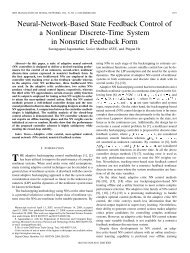
1858 IEEE TRANSACTIONS ON NEURAL NETWORKS, VOL. 22, NO. 12, DECEMBER 2011Fig. 1.J(e(k))v(k)Critic networkAction networku(k) = v(k) + u s(k)x(k+1) = f(x(k−σ 0),...,x(k−σ m))+g(x(k−σ 0),...,x(k−σ m))u(k)x(k+1)v(k)e(k)e(k)u s(k)e(k+1) = x(k+1) − η(k+1)Structure diagram of the algorithm.η(k+1) = s(η(k))η(k+1)IV. NEURAL NETWORK IMPLEMENTATION OF THEITERATION HDP ALGORITHMThe nonlinear optimal control solution relies on solving theHJB equation, exact solution of which is generally impossibleto be obtained for nonlinear time delay system. So we need touse parametric structures or neural networks to approximateboth control policy and performance index function. Therefore,in order to implement the HDP iterations, we employ neuralnetworks for approximations in this section.Assume the number of hidden layer neurons is denoted by l,the weight matrix between the input layer and hidden layer isdenoted by V , the weight matrix between the hidden layer andoutput layer is denoted by W, then the output of three-layerneural network is represented by( )ˆF(X, V, W) = W T σ V T X(64)where σ(V T X) ∈ R l is the sigmoid function. The gradientdescent rule is adopted for the weight update rules of eachneural network [26].Here, there are two networks, which are critic network andaction network, respectively. Both neural networks are chosenas three-layer BP network. The whole structure diagram isshowninFig.1.A. Critic NetworkThe critic network is used to approximate the performanceindex function J [i+1] (e(k)). The output of the critic networkis denoted as follows:( ) T ()Ĵ [i+1] (e(k)) = σ ) T e(k) . (65)w [i+1]c(v [i+1]cThe target function can be written as follows:J [i+1] (e(k)) = e T (k)Qe(k) + ( ˆv [i] (k) ) T R ˆv [i] (k)+Ĵ [i] (e(k + 1)). (66)Then we define the error function for the critic network asfollows:e c [i+1] (k) = Ĵ [i+1] (e(k)) − J [i+1] (e(k)). (67)The objective function to be minimized in the critic networkisE c [i+1] (k) = 1 (2e c (k)) [i+1] . (68)2So the gradient-based weights update rule for the criticnetwork is given bywherew c[i+2]v [i+2](k) = w c[i+1]c (k) = v c[i+1]w [i+1]cv [i+1]c(k) + w c[i+1] (k),(k) + v [i+1]c (k) (69)∂ E c(k) =−α [i+1] (k)c ,∂w c [i+1] (k)∂ E c(k) =−α [i+1]c∂v [i+1]c(k)(k)(70)and the learning rate α c of critic network is positive number.B. Action NetworkIn the action network, the states e(k − σ 0 ),...,e(k − σ m )are used as inputs to create the optimal control, ˆv [i] (k) asthe output of the network. The output can be formulated asfollows:( ) T ( )ˆv [i] (k) = w a[i] σ (v a [i] )T Y (k) (71)where Y (k) =[e T (k − σ 0 ),...,e T (k − σ m )] T .We define the output error of the action network as follows:e a [i] (k) =ˆv[i] (k) − v [i] (k). (72)The weights in the action network are updated to minimizethe following performance error measure:E a [i] (k) = 1 ( ) 2e a [i]2(k) . (73)The weights updating algorithm is similar to the one for thecritic network. By the gradient descent rule, we can obtainw a[i+1] (k) = w a [i] (k) + w a [i] (k),v a [i+1] (k) = v a [i] (k) + v a [i] (k) (74)wherew [i]a (k) =−α av [i]a (k) =−α a∂ E a [i] (k)∂w a [i] (k) ,∂ E [i]a (k)∂v [i]a (k)(75)and the learning rate α a of action network is positive number.V. SIMULATION STUDYIn this section, two examples are provided to demonstratethe effectiveness of the proposed iteration HDP algorithm inthis paper. One is about tracking chaotic signal, and the otheris about the situation that the function g(·) is noninvertible.
ZHANG et al.: OPTIMAL TRACKING CONTROL FOR A CLASS OF NONLINEAR DISCRETE-TIME SYSTEMS WITH TIME DELAYS BASED ON HDP 18591.511.51x 2η 2eta 20.50−0.5−1−1.5−1.5 −1 −0.5 0 0.5 1 1.5eta 1State trajectories0.50−0.5−1−1.50 10 20 30 40 50 60 70 80 90 100Time stepFig. 2.Hénon chaos orbits.Fig. 4. State variable trajectory x 2 and desired trajectory η 2 .State trajectories1.510.50−0.5−1−1.50 10 20 30 40 50 60 70 80 90 100Time stepx 1η 1Performance index function0.450.40.350.30.250.20.150.10.0500 5 10 15 20 25 30 35 40 45 50Iteration stepFig. 3. State variable trajectory x 1 and desired trajectory η 1 .Fig. 5.Convergence of performance index.A. Example 1Consider the following nonlinear time delay system whichis the example in [54] and [37] with modification:wherex(k + 1) = f (x(k), x(k − 1), x(k − 2))+ g(x(k), x(k − 1), x(k − 2))u(k)x(k) = ε 1 (k), −2 ≤ k ≤ 0 (76)f (x(k), x(k − 1), x(k − 2))[ 0.2x1 (k) exp (x=2 (k)) 2 ]x 2 (k − 2)0.3 (x 2 (k)) 2 x 1 (k − 1)and[ ]−0.2 0g(x(k), x(k − 1), x(k − 2)) =.0 −0.2The desired signal is well-known Hénon mapping as follows:[ ]η1 (k+1)η 2 (k+1)[1+b×η2 (k)−a×η1 2(k)η 1 (k)[ ]η1 (0)η 2 (0)=](77)where a = 1.4, b = 0.3,orbits are given as Fig. 2.Based on the implementation of proposed HDP algorithmin Section III-C, we first give the initial states as ε 1 (−2) =ε 1 (−1) = ε 1 (0) = [ 0.5 −0.5 ] T , and the initial control policyas β(k) = −2x(k). The implementation of the algorithmis at the time instant k = 3. The maximal iteration step= [ 0.1−0.1]. The chaotic signalError trajectories1.510.50−0.5−1−1.5−20 10 20 30 40 50 60 70 80 90 100Time stepFig. 6. Tracking error trajectories e 1 and e 2 .i max is 50. We choose three-layer BP neural networks asthe critic network and the action network with the structure2 − 8 − 1 and 6− 8 − 2, respectively. The iteration timeof the weights updating for two neural networks is 100.The initial weights are chosen randomly from [−0.1, 0.1],and the learning rate is α a = α c = 0.05. We selectQ = R = I 2 .The state trajectories are given as Figs. 3 and 4. The solidlines in the two figures are the system states, and the dashedlines are the trajectories of the desired chaotic signal. Fromthe two figures, we can see that the state trajectories of (76)follow the chaotic signal. From Lemma 2, Theorems 1 and 3,the performance index function sequence is bounded ande 1e 2
Page 1 and 2: IEEE TRANSACTIONS ON NEURAL NETWORK
Page 3: ZHANG et al.: OPTIMAL TRACKING CONT
Page 6: 1856 IEEE TRANSACTIONS ON NEURAL NE
Page 11 and 12: ZHANG et al.: OPTIMAL TRACKING CONT

Optimal Tracking Control for a Class of Nonlinear Discrete-Time ...

You also want an ePaper? Increase the reach of your titles

Delete template?

Save as template?