Electric Field and Electric Potential (B)

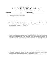
Pre-lab Quiz/PHYS 224Electric Field and Electric Potential (B)Your name___________ Lab section_______________ __1. What do you investigate in this lab?2. For two concentric conducting rings, the inner radius of the larger ring is 12.0 cm and the outerradius of the smaller ring is 4.0 cm. The electric potential of the inner ring is 0 and that of theouter ring is 10 V. Calculate the electric potential half way between the two rings, i.e., 8.0 cmaway from the center of the rings. (Answer: V=6.3 V)3. In the following figure, the electric potential of the inner conducting ring is 0 and the electricpotential of the outer conducing ring is −5.0 V. The two rings are concentric. Draw fourequipotential lines with 1 V-difference between two neighboring lines and label each line withthe corresponding voltage. Also draw four electric field lines in each figure.

Lab Report/PHYS 224Electric Field and Electric Potential (B)Name_ _________ Lab section_______________ __ObjectiveIn this lab, you study the electric field between two coaxial metal rings, map theequipotentials, determine the electric field, and plot the electric field lines. The electric field is notexact but resembles uniaxial electric field.BackgroundIn electrostatics, electric field ( E ) and electric potential (V) are two interchangeable physicalquantities for describing electric force, although the former is vector and the latter scalar.If placing a test electric charge of charge q at Point P in pace, it experiences an electric forcegiven by F qE , (1)where E is the electric field at Point P. When moving the test charge from Point P to Point Q, theelectric force on the charge varies proportionally with the electric field along the pathway. Thetotal work done by the electric force can be obtained by integrating the work along the pathway.Because the electrostatic force is conservative, the total work however depends only on the startingand ending points of the pathway but not on which specific pathway the charge traverses. One canthus introduce the electric potential difference between the two points which is related to the totalwork ( W ) done by the electric force , as described by equation W qV q( V QVP ) . (2)Therefore, if one maps out the electric field in space, one can calculate the electric potential inspace (apart from a common constant as the reference potential), and vice versa.As a vector quantity, electric field at a point must be described by its magnitude anddirection, altogether requiring three numbers. To visualize E in space, one normally draws electricfield lines (each line with an arrow to designate its direction) in space. The direction of E at apoint is parallel to the tangent of the electric field line passing through the point. The magnitude ofE at any point is proportional to the line density at the point.As a scalar quantity, electric potential at any point requires only one number to describe,apart from a common constant as the reference potential. As such, to plot electric potential inspace, one can simply find and draw equipotential surfaces (often simply referred asequipotentials). On each equipotential, the electric potential is the same at every point. Clearly, it ismuch easier to map and plot electric potential in space. Normally, one draws a series ofequipotentials, with the same potential difference between any two neighboring equipotentials. Toobtain electric field from the plot of equipotentials, one uses the following rules. At any point onan equipotential, the electric field must be perpendicular to the tangent of the equipotentialat that point, and electric field points from high potential to low potential. The magnitude ofthe electric field is inversely proportional to the distance between two neighboringequipotentials. If the potential difference between two infinitely close points B and A isV=V B −V A and the distance between A and B is d, the component of the electric fieldprojected in the direction pointing from A to B is given by E=−V/d.A uniaxial electric field can be induced between two concentric conducting cylindrical shells

a and b with their longitudinal lengths much larger compared to their separation. Assume the innerradius of the larger ring as r a and the outer radius of the smaller ring as r b . When an electricpotential difference ∆V 0 = V a −V b is established between the two rings, at any point between therings the electric field points radially and its magnitude depends only on the distance between thepoint and the symmetry axis of the rings. Use calculus, between the rings and at a distance of rfrom the symmetry axis of the rings, the magnitude of the electric field is given byCE , (3)rwhere the constant C V Vln( r / r ) . Thus, equipotentials are also concentric rings. Theab/a bpotential difference between two equipotentials is however not linearly proportional to theirdistance. Between the rings and at a distance of r from the symmetry axis of the rings, the electricpotential is given byV ( r) Vb C ln( r / rb) . (4)The SI units for the above equations are: E in volts per meter (V/m); d or r in meter(m); V in volt (V).EXPERIMENTApparatusFill the rectangular tray with 0.5-inch of water.Two metal rings are used as electrodes to studyuniaxially symmetric electric field. The outer diameterof the smaller ring is 1.9 in and the inner diameter ofthe larger ring is 6.0 in. Of the three point probes witha round supporting base, two (P1 and P2) are to beconnected to a DC power supply of 12 V and alsoconnected respectively to either pair of electrodes. Theother point probe (P3) and a hand-held point probe(P4) are used to map equipotentails. Because thelongitudinal lengths of the two metal rings are tooshort compared to their separation, the electric field between the two metal bars cannot beconsidered exactly as uniaxial. Therefore, as you will find, your measurements in this labshould not completely follow Equations (3) and (4).Procedures1. Set up the circuit (Figure 1)Place the circular graph paper underneath the tray. Place the two metal rings inside the tray,and align their centers with the center on the graph paper. Connect P1 to the ground of the DC powersupply and gently place its tip on the inner ring (the 0-V ring). Connect P2 to the positive terminalof the DC power supply and gently place its tip on the outer (bigger) ring (the 12-V ring). Note: thetips of P1 and P2 should be under the water surface and do not move the two rings again.Figure 2 displays only part of the circular graph paper (not to scale). Use the polar coordinates(r, ). Note: the labels 2, 4, and 6 in Figure 2 refer to the diameters (2r) of 2, 4, and 6 inches,and the unit for the r coordinate is inch.

Connect P2 to the positive lead of Voltmeter B and connect P3 to the negative lead ofVoltmeter B. Connect P3 to the positive lead of Voltmeter A and connect P4 to the negative lead ofVoltmeter B. Note: the sensitivity level of the voltmeters should be set properly. Place P3 and P4(their tips should be also under the water surface) inside the tray and between the two rings.Ask your TA to check the circuit!2. Investigate Electric Potential-versus-DistanceSet the output voltage (V a −V b ) of the DC power supply to 12 V. Turn off Voltmeter B, and turnon Voltmeter A. Place the tip of probe P3 at point (r=1.5 in, =0). Place the tip of probe P4 at pointswith =0 and in turn with r′=1.7, 1.9, 2.1, 2.3, and 2.5 in. Read the correspondingly potentialdifference (V) between the P4 and P3 from Voltmeter C. Record them in Table 1. Calculate V/(r′−r) and record the ratio values in Table 1. (Note: 1 inch= 0.0254 m.)TABLE 1r′ (inch) Potential difference V (V) V /(r−r′) (V/m)1.71.92.12.32.53. Map the first equipotentialTurn on only Voltmeter B. Move the tip of probe P3 to point (r=1.5, =0). Read its potentialfrom Voltmeter B. Mark the point in Figure 2. Record it in Table 2.Turn off Voltmeter B. Turn on Voltmeter A, and move the tip probe P4 along the =90° lineuntil Voltmeter A reads 0 V. This means that the tips of P3 and P4 are place on the sameequipotential. Read out the y coordinate of the tip of P4 and mark the point in Figure 2. Record it inTable 2.Repeat the measurement by moving the tip of P4 respectively along the =180° and 270° linesuntil Voltmeter A reads 0 V. Read out the corresponding r coordinates of the tip of P4 and mark thecorresponding points in Figure 2. Record them in Table 2. Draw a curve through the four points.Tip of P3(r=1.5, =0)potential(V)TABLE 2r′ for r′ for=90° =180°r′ for=270°Averager & r′(r=1.7, =0)(r=1.9, =0)(r=2.1, =0)(r=2.3, =0)(r=2.5, =0)

4. Map five more equipotentialsRepeat step 3 to map four more equipotentials by moving the tip of probe P3 respectively topoints (r=1.7 in, =0), (r=1.9 in, =0), (r=2.1 in, =0), (r=2.3 in, =0), and (r=2.5 in, =0).Questions1. For the measurement by step 2, should the measured V linearly proportional to r?2. Use arrow to mark the directions of the electric field at (r=2.0, =45°) and (r=2, =225°) inFigure 2.3. When using Equation (4) to describe the measured potential-versus-r, what are the valuesof r a , r b , V a , V b , and C?AnalysisCalculate the averaged r coordinate for the four points on each equipotential. Using theaveraged r coordinates and Equation (4) to calculate the corresponding potential. Record them inTable 1 and compare with the measured corresponding potentials.Using the averaged x coordinates and the measured corresponding potentials, calculate theaverage electric field values E V/ rbetween every two neighboring equipotentials. (Note: 1inch= 0.0254 m.)Between the 1 st and 2 nd : E Between the 2 nd and 3 rd : E Between the 3 rd and 4 th : E Between the 4 th and 5 th : E Between the 5 th and 6 th : E In Figure 2, draw four electric field lines.