Schaum's Outline Series

CHAPTER 3 Software Project Management 37
software developers aware of the significance of errors and error reduction. The
effects of changes in the software process can be seen in the error data.
Additionally, making the errors and error detection visible encourages testers
and developers to keep error reduction as a goal.
The error rate is the inverse of the inter-error time. That is, if errors occur every 2
days, then the instantaneous error rate is 0.5 errors/day. The current instantaneous
error rate is a good estimate of the current error rate. If the faults that cause errors
are not removed when the errors are found, then the cumulative error rate (the sum
of all the errors found divided by the total time) is a good estimate of future error
rates. Usually, most errors are corrected (the faults removed), and thus the error
rates should go down and the inter-error times should be increasing. Plotting this
data can show trends in the error rate (errors found per unit time). Fitting a straight
line to the points is an effective way to display the trend. The trend can be used to
estimate future error rates. When the trend crosses the x-axis, the estimate of the
error rate is zero, or there are no more errors. If the x-axis is number of errors, the
value of the x-intercept can be used as an estimate of the total number of errors in
the software. If the x-axis is the elapsed time of testing, the intercept is an estimate
of the testing time necessary to remove all errors. The area under this latter line is
an estimate of the number of errors originally in the software.
EXAMPLE 3.7
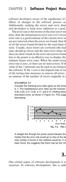
Consider the following error data (given as the times between errors): 4, 3, 5, 6, 4,
6, 7. The instantaneous error rates are the inverses of the inter-error times: 0.25,
0.33, 0.20, 0.17, 0.25, 0.17, and 0.14. Plotting these against error number gives a
downward curve, as shown in Figure 3-2. This suggests that the actual error rate is
decreasing.
Number of Errors
0.4
0.3
0.2
0.1
0
TEAMFLY
1 2 3 4 5 6 7 8 9 10 11 12 13
Error Rates
Fig. 3-2. Plot of error rates.
A straight line through the points would intersect the axis about 11. Since this
implies that the error rate would go to zero at the eleventh error, an estimate of the
total number of errors in this software would be 11 errors. Since seven errors have
been found, this suggests that there may be four more errors in the software.
3.9 Postmortem Reviews
One critical aspect of software development is to learn from your mistakes and
successes. In software development, this is called a postmortem. It consists of
Error