The Ball-Pivoting Algorithm for Surface Reconstruction - TAUBIN ...

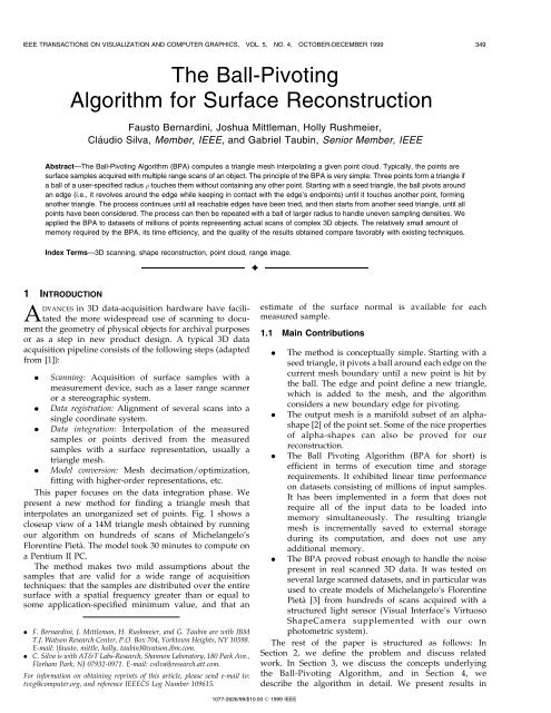
350 IEEE TRANSACTIONS ON VISUALIZATION AND COMPUTER GRAPHICS, VOL. 5, NO. 4, OCTOBER-DECEMBER 1999Fig. 1. Section of Michelangelo's Florentine PietaÁ. This 14M trianglemesh was generated from more than 700 scans using the ball pivotingalgorithm.Section 5, and discuss open problems and future work inSection 6.2 BACKGROUNDRecent years have seen a proliferation of scanningequipment and algorithms for synthesizing models fromscanned data. We refer the reader to two recent reviewsof research in the field [4], [5]. In this section, we focuson the role interpolating meshing schemes can play inscanning objects and why they have not been used inpractical scanning systems.2.1 Interpolating Meshes in Scanning SystemsWe define the scanning problem: Given an object, find acontinuous representation of the object surface that capturesfeatures of a length scale 2d or larger. The value of d isdictated by the application. Capturing features of scale 2drequires sampling the surface with a spatial resolution of dor less. The surface may consist of large areas that can bewell approximated by much sparser meshes; however, inthe absence of a priori information, we need to begin with asampling resolution of d or less to guarantee that no featureis missed.We consider acquisition systems that produce sets ofrange images, i.e., arrays of depths, each of which covers asubset of the full surface. Because they are height fields withregular sampling, individual range images are easilymeshed. The individual meshes can be used to computean estimated surface normal for each sample point.An ideal acquisition system would return samples lyingexactly on the object surface, but any real measurementsystem introduces some error. However, if a system returnssamples with an error that is orders of magnitude smallerthan the minumum feature size, the sampling can beregarded as perfect. A surface can then be reconstructed byfinding an interpolating mesh without additional operationson the measured data. Most scanning systems stillneed to account for acquisition error. There are two sourcesof error: error in registration; and error along the sensor lineof sight. Estimates of actual surface points are usuallyderived by averaging samples from redundant scans. Theseestimates are then connected into a triangle mesh.Most methods for estimating surface points depend ondata structures that facilitate the construction of the mesh.Two classes of methods have been used successfully forlarge datasets; both assume negligible registration errorand compute estimates to correct for line-of-sight error.The first of these classes is volumetric methods, such asthat introduced by Curless and Levoy [6]. In thesemethods, individual aligned meshes are used to computea signed-distance function on a volume grid encompassingthe object. Estimated surface points are computed asthe points on the grid where the distance funtion is zero.The structure of the volume then facilitates the constructionof a mesh using the marching cubes algorithm [7].The second class of methods are mesh stitching methods,such as the technique of Soucy and Laurendeau [8]. Disjointheight-field meshes are stitched into a single surface.Disjoint regions are defined by finding areas of overlap ofdifferent subsets of the set of scans. Estimated surfacepoints for each region are computed as weighted averagesof points from the overlapping scans. Estimated points ineach region are then re-triangulated, and the resultingmeshes are stitched into a single mesh. Turk and Levoydeveloped a similar method [9], which first stitches (orzippers) the disjoint meshes and then computes estimatedsurface points.We observe that in both cases of methods, the method ofestimating surface points need not be so closely linked tothe method for constructing the final mesh. In thevolumetric approach, a technique other than marchingcubes could be used for finding a triangle mesh passingthrough the estimated surface points. In the mesh-joiningapproaches, a technique for finding a mesh connecting allestimated surface points could be used in place of stitchingtogether the existing meshes. Most importantly, with anefficient algorithm for computing a mesh which joinspoints, any method for computing estimated surface pointscould be used, including those that do not imposeadditional structure on the data and do not treat registrationand line-of-sight error separately. For example, it has beendemonstrated that reducing error in individual meshesbefore alignment can reduce registration error [10].We are developing a method that moves sampleswithin known scanner error bounds to conform themeshes to one another as they are aligned. Our currentimplementation of this method was used to preprocessthe data shown in the results section. The method will bedescribed in a future paper.Finally, it may be desirable to find an interpolating meshfrom measured data even if it contains uncompensatederror. The preliminary mesh could be smoothed, cleaned,and decimated for use in planning functions. A meshinterpolating measured points could also be used as astarting point for computing consensus points.2.2 State of the Art for Interpolating MeshesExisting interpolating techniques fall into two categories:sculpting-based [11], [12], [4] and region-growing [13],[14], [15], like the BPA. In sculpting-based methods, a

BERNARDINI ET AL.: THE BALL-PIVOTING ALGORITHM FOR SURFACE RECONSTRUCTION 351volume tetrahedralization is computed from the datapoints, typically the 3D Delaunay triangulation. Tetrahedraare then removed from the convex hull to extractthe original shape. Region-growing methods start with aseed triangle, consider a new point and join it to theexisting region boundary, and continue until all pointshave been considered.The strength of sculpting-based approaches is that theyoften provide theoretical guarantees for the quality of theresulting surface, e.g., that the topology is correct and thatthe surface converges to the true surface as the samplingdensity increases (see e.g., [16], [17]). However, computingthe required 3D Delaunay triangulation can be prohibitivelyexpensive in terms of time and memory required and canlead to numerical instability when dealing with datasets ofmillions of points. The goal of the BPA is to retain thestrengths of previous interpolating techniques in a methodthat exhibits linear time complexity and robustness on realscanned data.3 SURFACE RECONSTRUCTION AND BALL-PIVOTINGThe main concept underlying the Ball-Pivoting Algorithm isquite simple. Let the manifold M be the surface of a threedimensionalobject and S be a point-sampling of M. Let usassume for now that S is dense enough that a -ball (a ballof radius ) cannot pass through the surface withouttouching sample points (see Fig. 3 for a 2D example). Westart by placing a -ball in contact with three sample points.Keeping the ball in contact with two of these initial points,we ªpivotº the ball until it touches another point, asillustrated in Fig. 2 (more details are given in Section 4.3).We pivot around each edge of the current mesh boundary.Triplets of points that the ball contacts form new triangles.The set of triangles formed while the ball ªwalksº on thesurface constitutes the interpolating mesh.The BPA is closely related to alpha-shapes [18], [2]. Infact every triangle computed by the -ball walk obviouslyhas an empty smallest open ball b whose radius is less than (see [2], page 50). Thus, the BPA computes a subset of the2-faces of the -shape of S. These faces are also a subset ofthe 2-skeleton of the three-dimensional Delaunay triangulationof the point set. Alpha shapes are an effective tool forcomputing the ªshapeº of a point set. The surfacereconstructed by the BPA retains some of the qualities ofalpha-shapes: It has provable reconstruction guaranteesunder certain sampling assumptions, and an intuitivelysimple geometric meaning.However, the 2-skeleton of an alpha-shape computedfrom a noisy sampling of a smooth manifold can containmultiple nonmanifold connections. It is nontrivial to filterout unwanted components. Also, in their original formulation,alpha-shapes are computed by extracting asubset of the 3D Delaunay triangulation of the point set, adata structure that is not easily computed for datasets ofmillions of points. With the assumptions on the inputstated in the introduction, the BPA efficiently androbustly computes a manifold subset of an alpha-shapethat is well suited for this application.In [16], sufficient conditions on the sampling density of acurve in the plane were derived which guarantee that theFig. 2. Ball pivoting operation. See Section 4.3 for further details.The pivoting ball is in contact with the three vertices of triangle ˆ… i ; j ; o †, whose normal is n. The pivoting edge e …i;j† lies onthe z axis (perpendicular to the page and pointing towards theviewer), with its midpoint m at the origin. The circle s ijo is theintersection of the pivoting ball with z ˆ 0. The coordinate frame issuch that the center c ijo of the ball lies on the positive x axis.During pivoting, the -ball stays in contact with the two edgeendpoints i ; j , and its center describes a circular trajectory withcenter in m and radius jjc ijo mjj. In its pivoting motion, the ballhits a new data point k . Let s k be the intersection of a -spherecentered at k with z ˆ 0. The center c k of the pivoting ball when ittouches k is the intersection of with s k lying on the negativehalfplane of oriented line l kalpha-shape reconstruction is homeomorphic to the originalmanifold and that it lies within a bounded distance. Thetheorem can be easily extended to surfaces (stated herewithout proof): suppose that for the smooth manifold M,the sampling S satisfies the following properties:1. The intersection of any ball of radius with themanifold is a topological disk.2. Any ball of radius centered on the manifoldcontains at least one sample point in its interior.The first condition guarantees that the radius ofcurvature of the manifold is larger than , and that the-ball can also pass through cavities and other concavefeatures without multiple contacts with the surface. Thesecond condition tells us that the sampling is denseenough that the ball can walk on the sample pointswithout leaving holes (see Fig. 3 for 2D examples). TheBPA then produces a homeomorphic approximation T ofthe smooth manifold M. We can also define a homeomorphismh : T7!M such that the distance jjp h…p†jj

352 IEEE TRANSACTIONS ON VISUALIZATION AND COMPUTER GRAPHICS, VOL. 5, NO. 4, OCTOBER-DECEMBER 1999Fig. 3. The Ball Pivoting Algorithm in 2D. (a) A circle of radius pivots from sample point to sample point, connecting them with edges. (b) When thesampling density is too low, some of the edges will not be created, leaving holes. (c) When the curvature of the manifold is larger than 1=, some ofthe sample points will not be reached by the pivoting ball, and features will be missed.The BPA is designed to process the output of an accurateregistration/conformance algorithm (see Section 2), anddoes not attempt to average out noise or residualregistration errors. Nonetheless, the BPA is robust in thepresence of imperfect data.We augment the data points with approximate surfacenormals computed from the range maps to disambiguatecases that occur when dealing with missing or noisy data.For example, if parts of the surface have not been scanned,there will be holes larger than in the sampling. It is thenimpossible to distinguish an interior and an exterior regionwith respect to the sampling. We use surface normals (forwhich we assume outward orientation) to decide surfaceorientation. For example, when choosing a seed triangle wecheck that the surface normals at the three vertices areconsistently oriented.Areas of density higher than present no problem. Thepivoting ball will still ªwalkº on the points forming smalltriangles. If the data is noise-free and is smaller than thelocal curvature, all points will be interpolated. More likely,points are affected by noise and some of those lying belowthe surface will not be touched by the ball and will not bepart of the reconstructed mesh (see Fig. 4a).Missing points create holes that cannot be filled by thepivoting ball. Any postprocessing hole-filling algorithmcould be employed; in particular, BPA can be appliedmultiple times, with increasing ball radii, as explained inSection 4.6. However, we do need to handle possibleambiguities that missing data can introduce. When pivotingaround a boundary edge, the ball can touch an unusedpoint lying close to the surface. Again, we use surfacenormals to decide whether the point touched is valid or not(see Fig. 4b). A triangle is rejected if the dot product of itsnormal with the surface normal is negative.The presence of misaligned overlapping range scanscan lead to poor results if the registration error is similarto the pivoting ball size. Undesired small connectedcomponents lying close to the main surface will beformed, and the main surface will be affected by highfrequency noise (see Fig. 4c). Our seed selection strategyavoids creating a large number of such small components.A simple postprocessing that removes small componentsand surface smoothing [19] can significantly improve theresult in these cases, at least aesthetically.Regardless of the defects in the data, the BPA isguaranteed to build an orientable manifold. Notice thatthe BPA will always try to build the largest possibleconnected manifold from a given seed triangle.Choosing a suitable value for the radius of the pivotingball is typically easy. Current structured-light or lasertriangulation scanners produce very dense samplings,exceeding our requirement that intersample distance beFig. 4. Ball pivoting in the presence of noisy data. (a) Surface samples lying ªbelowº surface level are not touched by the pivoting ball and remainisolated (and are discarded by the algorithm). (b) Due to missing data, the ball pivots around an edge until it touches a sample that belongs to adifferent part of the surface. By checking that triangle and data point normals are consistently oriented, we avoid generating a triangle in this case. (c)Noisy samples form two layers, distant enough to allow the ball to ªwalkº on both layers. A spurious small component is created. Our seed selectionstrategy avoids the creation of a large number of these small components. Remaining ones can be removed with a simple postprocessing step. In allcases, the BPA outputs an orientable, triangulated manifold.

BERNARDINI ET AL.: THE BALL-PIVOTING ALGORITHM FOR SURFACE RECONSTRUCTION 353less than half the size of features of interest. Knowledge ofthe sampling density characteristics of the scanner, and ofthe feature size one wants to capture, are enough to choosean appropriate radius. Alternatively, one could analyze asmall subset of the data to compute the point density. Anuneven sampling might arise when scanning a complexsurface with regions that project into small areas in thescanner direction. The best approach is to take additionalscans with the scanner perpendicular to such regions toacquire additional data. Notice, however, that the BPA canbe applied multiple times, with increasing ball radii, tohandle uneven sampling densities, as described inSection 4.6.4 THE BALL-PIVOTING ALGORITHMThe BPA follows the advancing-front paradigm to incrementallybuild an interpolating triangulation. BPA takes asinput a list of surface-sample data points i , each associatedwith a normal n i (and other optional attributes, such astexture coordinates), and a ball radius . The basicalgorithm works by finding a seed triangle (i.e., three datapoints … i ; j ; k † such that a ball of radius touching themcontains no other data point) and adding one triangle at atime by performing the ball pivoting operation introducedin Section 3.The front F is represented as a collection of linked lists ofedges and is initially composed of a single loop containingthe three edges defined by the first seed triangle. Each edgee …i;j† of the front is represented by its two endpoints … i ; j †,the opposite vertex o , the center c ijo of the ball that touchesall three points, and links to the previous and next edgealong in the same loop of the front. An edge can be active,boundary, orfrozen. Anactive edge is one that will be usedfor pivoting. If it is not possible to pivot from an edge, it ismarked as boundary. The frozen state is explained below, inthe context of our out-of-core extensions. Keeping all thisinformation with each edge makes it simpler to pivot theball around it. The reason the front is a collection of linkedlists, instead of a single one, is that as the ball pivots alongan edge, depending on whether it touches a newlyencountered data point or a previously used one, the frontchanges topology. BPA handles all cases with two simpletopological operators, join and glue, which ensure that atany time the front is a collection of linked lists.The basic BPA algorithm is shown in Fig. 5. Below wedetail the functions and data structures used. In particular,we later describe a simple modification necessary to thebasic algorithm to support efficient out-of-core execution.This allows BPA to triangulate large datasets with minimalmemory usage.4.1 Spatial QueriesBoth ball_pivot and find_seed_triangle (lines 3 and 10 inFig. 5) require efficient lookup of the subset of pointscontained in a small spatial neighborhood. We implementedthis spatial query using a regular grid of cubiccells, or voxels. Each voxel has sides of size ˆ 2. Datapoints are stored in a list, and the list is organized usingbucket-sort so that points lying in the same voxel form acontiguous sublist. Each voxel stores a pointer to theFig. 5. Skeleton of the BPA algorithm. Several necessary error testshave been left out for readability, such as edge orientation checks. Theedges in the front F are generally accessed by keeping a queue ofactive edges. The join operation adds two active edges to the front. Theglue operation deletes two edges from the front, and changes thetopology of the front by breaking a single loop into two, or combining twoloops into one. See text for details. The find_seed_triangle functionreturns a -exposed triangle, which is used to initialize the front.beginning of its sublist of points (to the next sublist if thevoxel is empty). An extra voxel at the end of the gridstores a NULL pointer. To visit all points in a voxel it issufficient to traverse the list from the node pointed to bythe voxel to the one pointed to by the next voxel.Given a point p, we can easily find the voxel V it liesin by dividing its coordinates by . We usually need tolook up all points within 2 distance from p, which are asubset of all points contained in the 27 voxels adjacent toV (including V itself).The grid allows constant-time access to the points. Itssize would be prohibitive if we processed a large dataset inone step; but an out-of-core implementation, described inSection 4.5, can process the data in manageable chunks.Memory usage can be further reduced, at the expense of aslower access, using more compact representations, such asa sparse matrix data structure.4.2 Seed SelectionGiven data satisfying the conditions of the reconstructiontheorem of Section 3, one seed per connected componentis enough to reconstruct the entire manifold (functionfind_seed_triangle at line 10 in Fig. 5). A simple way tofind a valid seed is to:. Pick any point not yet used by the reconstructedtriangulation.. Consider all pairs of points a ; b in its neighborhoodin order of distance from .. Build potential seed triangles ; a ; b .

354 IEEE TRANSACTIONS ON VISUALIZATION AND COMPUTER GRAPHICS, VOL. 5, NO. 4, OCTOBER-DECEMBER 1999. Check that the triangle normal is consistent with thevertex normals, i.e., pointing outward.. Test that a -ball with center in the outwardhalfspace touches all three vertices and contains noother data point.. Stop when a valid seed triangle has been found.In the presence of noisy, incomplete data, it is important toselect an efficient seed-searching strategy. Given a validseed, the algorithm builds the largest possible connectedcomponent containing the seed. Noisy points lying at adistance slightly larger than 2 from the reconstructedtriangulation could form other potential seed triangles,leading to the construction of small sets of triangles lyingclose to the main surface (see Fig. 4c). These smallcomponents are an artifact of the noise present in the dataand are usually undesired. While they are easy to eliminateby postfiltering the data, a significant amount of computationalresources is wasted in constructing them.We can, however, observe the following: If we limitourselves to considering only one data point per voxel as acandidate vertex for a seed triangle, we cannot misscomponents spanning a volume larger than a few voxels.Also, for a given voxel, consider the average normal n ofpoints within it. This normal approximates the surfacenormal in that region. Since we want our ball to walk ªonºthe surface, it is convenient to first consider points whoseprojection onto n is large and positive.We therefore simply keep a list of nonempty voxels. Wesearch these voxels for valid seed triangles, and when one isfound, we start building a triangulation using pivotingoperations. When no more pivoting is possible, we continuethe search for a seed triangle from where we had stopped,skipping all voxels containing a point that is now part of thetriangulation. When no more seeds can be found, thealgorithm stops.4.3 Ball PivotingA pivoting operation (line 3 in Fig. 5) starts with a triangle ˆ… i ; j ; o † and a ball of radius that touches its threevertices. Without loss of generality, assume edge e …i;j† is thepivoting edge. The ball in its initial position (let c ijo be itscenter) does not contain any data point, either because is aseed triangle, or because was computed by a previouspivoting operation. The pivoting is in principle a continuousmotion of the ball, during which the ball stays incontact with the two endpoints of e …i;j† , as illustrated inFig. 2. Because of this contact, the motion is constrained asfollows: The center c ijo of the ball describes a circle whichlies on the plane perpendicular to e …i;j† and through itsmidpoint m ˆ 12 … j ‡ i ). The center of this circular trajectoryis m and its radius is jjc ijo mjj. During this motion,the ball may hit another point k . If no point is hit, then theedge is a boundary edge. Otherwise, the triangle … i ; k ; j †is a new valid triangle, and the ball in its final position doesnot contain any other point, thus being a valid starting ballfor the next pivoting operation.In practice, we find k as follows: We consider all pointsin a 2-neighborhood of m. For each such point x , wecompute the center c x of the ball touching i ; j and x ,ifsuch a ball exists. Each c x lies on the circular trajectory around m and can be computed by intersecting a -spherecentered at x with the circle . Of these points c x , we selectthe one that is first along the trajectory . We report the firstpoint hit and the corresponding ball center. Trivial rejectiontests can be added to speed up finding the first hit-point.4.4 The Join and Glue OperationsThese two operations generate triangles while adding andremoving edges from the front loops (lines 5-7 in Fig. 5).The simpler operation is the join, which is used when theball pivots around edge e …i;j† , touching a not_used vertex k(i.e., k is a vertex that is not yet part of the mesh). In thiscase, we output the triangle … i ; k ; j †, and locally modifythe front by removing e …i;j† and adding the two edges e …i;k†and e …k;j† (see Fig. 6).When k is already part of the mesh, one of two cases canarise:1. k is an internal mesh vertex, (i.e., no front edge uses k ). The corresponding triangle cannot be generated,since it would create a nonmanifold vertex. In thiscase, e …i;j† is simply marked as a boundary edge;2. k belongs to the front. We first check that addingthe candidate new triangle would not create anonmanifold or nonorientable manifold. This iseasily accomplished by looking at the existenceand orientation of edges incident on k . Then weapply a join operation, and output the new meshtriangle … i ; k ; j †. The join could potentially create(one or two) pairs of coincident edges (with oppositeorientation), which are removed by the glueoperation.The glue operation removes from the front pairs ofcoincident edges, with opposite orientation (coincidentedges with the same orientation are never created by thealgortihm). For example, when edge e …i;k† is added to thefront by a join operation (the same applies to e …k;j† ), if edgee …k;i† is on the front, glue will remove the pair of edgese …i;k† ;e …k;i† and adjust the front accordingly. Four cases arepossible, as illustrated in Fig. 7.A sequence of join and glue operations is illustrated inFig. 8.4.5 Out-of-Core ExtensionsBeing able to use a personal computer to triangulate highresolutionscans allows inexpensive on-site processing ofdata. Due to their locality of reference, advancing-frontalgorithms are suited to very simple out-of-core extensions.We employed a simple data-slicing scheme to extend thealgorithm shown in Fig. 5. The basic idea is to cache theportion of the dataset currently being used for pivoting, todump data no longer being used, and to load data as it isneeded. In our case, we use two axis-aligned planes 0 andto define the active region of work for pivoting. We 1initially place 0 in such a way that no data points lieªbelowº it, and 1 above 0 at some user-specified distance.As each edge is created, we test if its endpoints are ªaboveº 1 ; in this case, we mark the edge frozen. When all edgesremaining in the queue are frozen, we simply shift 0 and 1ªupwardsº, and update all frozen into active edges, and soon. A subset of data points is loaded and discarded from

BERNARDINI ET AL.: THE BALL-PIVOTING ALGORITHM FOR SURFACE RECONSTRUCTION 355Fig. 6. A join operation simply adds a new triangle, removing edgee …i;j† from the front and adding the two new edges e …i;k† and e …k;j† .memory when the corresponding bounding box enters andexits the active slice. Scans can easily be preprocessed tobreak them up into smaller meshes, so that they span only afew slices, and memory load remains low.The only change required in the algorithm to implementthis refinement is an outer loop to move the active slice, andthe addition of the instructions to unfreeze edges betweenlines 1-2 of Fig. 5.4.6 Multiple PassesTo deal with unevenly sampled surfaces, we can easilyextend the algorithm to run multiple passes with increasingFig. 8. Example of a sequence of join and glue operations. (a) A newtriangle is to be added to the existing front. The four front vertices insidethe dashed circle all represent a single data point. (b) A join removes anedge and creates two new front edges, coincident with existing ones. (c),(d) Two glue operations remove coincident edge pairs. (d) Also showsthe next triangle added. (e) Only one of the edges created by this join iscoincident with an existing edge. (f) One glue removes the duplicatepair.ball radii. The user specifies a list of radii f 0 ; ...; n g as input parameters. In each slice, for increasing i ;iˆ 0; ...;n, we start by inserting the points in a grid ofvoxel size ˆ 2 i . We let BPA run until there are no moreactive edges in the queue. At this point we increment i, gothrough all front edges, and check whether each edge withits opposite vertex o forms a valid seed triangle for a ball ofradius i . If it is, then it is added to the queue of activeedges. Finally, the pivoting is started again.Fig. 7. A glue operation is applied when join creates an edge identical toan existing edge, but with opposite orientation. The two coincidentedges are removed and the front adjusted accordingly. There are fourpossible cases: (a) The two edges form a loop. The loop is deleted fromthe front. (b) Two edges belong to the same loop and are consecutive.The edges are removed and the loop shortened. (c) The edges are notconsecutive and they belong to the same loop. The loop is split into two.(d) The edges are not consecutive and belong to two different loops. Theloops are merged into a single loop.4.7 RemarksThe BPA algorithm was implemented in C++ using theStandard Template Library. The whole code is less than4,000 lines, including the out-of-core extensions.The algorithm is linear in the number of data points anduses linear storage, under the assumption that the datadensity is bounded. This assumption is appropriate forscanned data, which is collected by equipment with aknown sample spacing. Even if several scans overlap, thetotal number of points in any region will be bounded by aknown constant.Most steps are simple O…1† state checks or updates toqueues, linked lists, and the like. With bounded density, apoint need only be related to a constant number ofneighbors. So, for example, a point can only be containedin a constant number of loops in the advancing front. Thetwo operations ball_pivot and find_seed_triangle are morecomplex.Each ball_pivot operates on a different mesh edge, so thenumber of pivots is O…n†. A single pivot requires identifyingall points in a 2 neighborhood. A list of these pointscan be collected from 27 voxels surrounding the candidate

356 IEEE TRANSACTIONS ON VISUALIZATION AND COMPUTER GRAPHICS, VOL. 5, NO. 4, OCTOBER-DECEMBER 1999point in our grid. With bounded density, this list hasconstant size B. We perform a few algebraic computationson each point in the list and select the minimum result, allO…1† operations on a list of size O…1†.Each find_seed_triangle picks unused points one at a timeand tests whether any incident triangle is a valid seed. Nopoint is considered more than once, so this test is performedonly O…n† times. To test a candidate point, we gather thesame point-list discussed above, and consider pairs ofpoints until we either find a seed triangle or reject thecandidate. Testing one of these triangles may requireclassifying every nearby point against a sphere touchingthe three vertices, in the worst case, O…B 3 †ˆO…1† steps. Inpractice, we limit the number of candidate points andtriangles tested by the heuristics discussed in Section 4.2.An in-core implementation of the BPA uses O…n ‡ L†memory, where L is the number of cells in the voxel grid.The O…n† term includes the data, the advancing front(which can only include each mesh edge once), and thecandidate edge queue. Our out-of-core implementationuses O…m ‡ L 0 † memory, where m is the number of datapoints in the largest slice and L 0 is the size of the smallergrid covering a single slice. Since the user can control thesize of slices, memory requirements can be tailored to theavailable hardware. The voxel grid can be more compactlyrepresented as a sparse matrix, with a small(constant) increase in access time.5 EXPERIMENTAL RESULTSOur experiments for this paper were all conducted on one450MHz Pentium II Xeon processor of an IBM IntelliStationZ Pro running Windows NT 4.0.In our experiments we used several datasets: ªcleanºdataset (i.e., points from analytical surface, see Fig. 9); thedatasets from the Stanford scanning database (seeFigs. 11a-c); and a very large dataset we acquired ourselves(and the main motivation of this work), a model ofMichelangelo's Florentine PietaÁ [3] (see Fig. 11d).To allow flexible input of multiple scans and out-of-coreexecution, our program reads its input in four parts: A listof individual scans to be converted into a single coherentFig. 9. Results. Triangle mesh computed by the BPA interpolating pointstriangle mesh; and for each scan, a transformation matrix, aposttransform bounding box (used to quickly estimate themesh position for assignment to a slice), and the actual scan,which is loaded only when needed.5.1 ExperimentsThe table in Fig. 10 summarizes our results. The ªcleanºdataset is a collection of points from an analytical surface.The Stanford Bunny, Dragon and Buddha datasets aremultiple laser range scans of small objects. The scannerused to acquire the data was a CyberWare 3030MS.These data required some minor preprocessing. We usedthe Stanford vrip program to connect the points within eachindividual range data scan to provide estimates of surfacenormals. We also removed the plane carvers, large planes oftriangles used for hole-filling by algorithms described in [6].Fig. 10. Summary of results. # of Pts and # of Scans are the original number of data points and range images respectively. lists the radii of thepivoting balls, in mm. Multiple radii mean that multiple passes of the algorithm, with increasing ball size, were used. # Slices is the number of slicesinto which the data is partitioned for out-of-core processing. # of Triangles is the number of triangles created by BPA. Mem. Usage is the maximumamount of memory used at any time during mesh generation, in MB. I/O Time is the time spent reading the input binary files; it also includes the timeto write the output mesh, as an indexed triangle set, in binary format. CPU Time is the time spent computing the triangulation. All times are inminutes, except where otherwise stated. All tests were performed on a 450MHz Pentium II Xeon.

BERNARDINI ET AL.: THE BALL-PIVOTING ALGORITHM FOR SURFACE RECONSTRUCTION 357Fig. 11. Results. (a) Stanford bunny. (b) Stanford dragon. (c) Stanford Buddha. (d) Preliminary reconstruction of Michelangelo's Florentine PietaÁ.This change was made only for aesthetic reasons; BPA hasno problem handling the full input.In order to confirm the effectiveness of our out-of-corecapabilities, we modified the Stanford Dragon bysubdividing each range mesh into several pieces,multiplying the original 71 meshes to over 1,452. A similarpreprocessing was also applied to the Buddha dataset. Wenote that such decompositions can be performed efficientlyfor arbitrarily large range scans (which do not necessarilyneed to fit in memory) by the techniques described in [20].The PietaÁ data has undergone extensive preprocessingduring and after scanning and registration that is out of thescope of this paper. The data is large enough that it cannotbe processed in-core, and is only processed in slices. Thescanning of the PietaÁ also included the capture of multiplecolor images with calibrated lighting, from which

358 IEEE TRANSACTIONS ON VISUALIZATION AND COMPUTER GRAPHICS, VOL. 5, NO. 4, OCTOBER-DECEMBER 1999reflectance and normals maps to augment the geometricdata are computed (see [21]).6 CONCLUSIONSIn this paper, we introduced the Ball-Pivoting Algorithm,an advancing-front algorithm to incrementally build aninterpolating triangulation of a given point cloud. BPA hasseveral desirable properties:. Intuitive: BPA triangulates a set of points byªrollingº a -ball on the point cloud. The userchooses only a single parameter.. Flexible, efficient, and robust: Our test datasetsranged from small synthetic data to large real worldscans. We have shown that our implementation ofBPA works on datasets of millions of pointsrepresenting actual scans of complex 3D objects.For our PietaÁ data, we found that on a Pentium II PCthe algorithm generates and writes to disk the outputmesh at a rate of roughly 500K triangles per minute.. Theoretical foundation: BPA is related toalpha-shapes [2], and given sufficiently densesampling, it is guaranteed to reconstruct a surfacehomeomorphic to and within a bounded distancefrom the original manifold.There are some avenues for further work. It would beinteresting to evaluate whether BPA can be used totriangulate surfaces sampled with particle systems. Thispossibility was left as an open problem in [22], and furtherdeveloped in [23] in the context of isosurface generation.By using weighted points, we might be able to generatetriangulations of adaptive samplings. The sampling densitycould be changed depending on local surface properties,and point weights accordingly assigned or computed. Anextension of our algorithm along the lines of the weightedgeneralization of alpha-shapes [18] should be able togenerate a more compact, adaptive, interpolatingtriangulation.We have done some initial experiments in using asmoothing algorithm adapted from [19] to preprocess thedata and to compute consensus points from multipleoverlapping scans to be used as input to the BPA, whileat the same time making small refinements to the rigidalignment of the scans to each other. Datasets used in thispaper were preprocessed using our current implementationof this algorithm.ACKNOWLEDGMENTSThe authors would like to thank the Stanford UniversityComputer Graphics Laboratory for making some of therange data used in this paper publicly available. Theywould also like to thank the Museo dell'Opera del Duomoin Florence, Italy for their kind collaboration in allowingthem to scan Michelangelo's PietaÁ and Dr. Jack Wassermanfor proposing and collaborating on the project.REFERENCES[1] K. Pulli, T. Duchamp, H. Hoppe, J. McDonald, L. Shapiro,and W. Stuetzle, ªRobust Meshes from Multiple RangeMaps,º Intl. Conf. Recent Advances in 3D Digital Imaging andModeling, pp. 205-211, IEEE CS Press, May 1997.[2] H. Edelsbrunner and E.P. MuÈ cke, ªThree-Dimensional AlphaShapes,º ACM Trans. Graph., vol. 13, no. 1, pp. 43-72, Jan. 1994.[3] J. Abouaf, ªThe Florentine PietaÁ: Can Visualization Solve the450-year-old Mystery?,º IEEE Computer Graphics & Applications,vol. 19, no. 1, pp. 6±10, Feb. 1999.[4] F. Bernardini, C. Bajaj, J. Chen, and D. Schikore, ªAutomaticReconstruction of 3D CAD Models from Digital Scans,º Int'lJ. Computational Geometry and Applications, vol. 9, nos. 4 & 5,pp. 327-370, Aug.-Oct. 1999.[5] R. Mencl and H. MuÈ ller, ªInterpolation and Approximation ofSurfaces from Three-Dimensional Scattered Data Points,º Proc.Eurographics '98, Eurographics, State of the Art Reports, 1998.[6] B. Curless and M. Levoy, ªA Volumetric Method for BuildingComplex Models from Range Images,º Proc. SIGGRAPH '96Computer Graphics Conf., pp. 303-312, 1996.[7] W. Lorensen and H. Cline, ªMarching Cubes: A High Resolution3D Surface Construction Algorithm,º Computer Graphics, vol. 21,no. 4, pp. 163-170, 1987.[8] M. Soucy and D. Laurendeau, ªA General Surface Approach to theIntegration of a Set of Range Views,º IEEE Trans. Pattern Analysisand Machine Intelligence, vol. 17, no. 4, pp. 344-358, Apr. 1995.[9] G. Turk and M. Levoy, ªZippered Polygonal Meshes fromRange Images,º Proc. SIGGRAPH '94 Computer Graphics Conf.,pp. 311-318, 1994.[10] C. Dorai, G. Wang, A.K. Jain, and C. Mercer, ªRegistration andIntegration of Multiple Object Views for 3D Model Construction,ºIEEE Trans. Pattern Analysis and Machine Intelligence, vol. 20, no. 1,pp. 83-89, Jan. 1998.[11] C. Bajaj, F. Bernardini, and G. Xu, ªAutomatic Reconstruction ofSurfaces and Scalar Fields from 3D Scans,º Proc. SIGGRAPH '95Computer Graphics Conf., pp. 109-118, 1995.[12] N. Amenta, M. Bern, and M. Kamvysselis, ªA New Voronoi-BasedSurface Reconstruction Algorithm,º Proc. SIGGRAPH '98 ComputerGraphics Conf., pp. 415-412, 1998.[13] J.-D. Boissonnat, ªGeometric Structures for Three-DimensionalShape Representation,º ACM Trans. Graph., vol. 3, no. 4, pp. 266-286,1984.[14] R. Mencl, ªA Graph-Based Approach to Surface Reconstruction,ºProc. EUROGRAPHICS '95, Computer Graphics Forum, vol. 14, no. 3,pp. 445-456, 1995.[15] A. Hilton, A. Stoddart, J. Illingworth, and T. Windeatt, ªMarchingTriangles: Range Image Fusion for Complex Object Modelling,ºProc. IEEE Int'l Conf. Image Processing, vol. 2, pp. 381-384,Laussane, 1996.[16] F. Bernardini and C. Bajaj, ªSampling and ReconstructingManifolds Using Alpha-Shapes,º Proc. Ninth Canadian Conf.Computational Geometry, pp. 193-198, Aug. 1997. Updated onlineversion available at www.qucis.queensu.ca/cccg97.[17] N. Amenta and M. Bern, ªSurface Reconstruction by VoronoiFiltering,º Proc. 14th Ann. ACM Symp. Computer Geometry, pp. 39-48, 1998.[18] H. Edelsbrunner, ªWeighted Alpha Shapes,º Technical ReportUIUCDCS-R-92-1,760, Computer Science Dept., Univ. Illinois,Urbana, IL, 1992.[19] G. Taubin, ªA Signal Processing Approach to Fair Surface Design,ºProc. ACM SIGGRAPH '95 Computer Graphics Conf., pp. 351-358,Aug. 1995.[20] Y.-J. Chiang, C.T. Silva, and W. Schroeder, ªInteractive Outof-CoreIsosurface Extraction,º Proc. IEEE Visualization '98,pp. 167-174, Nov. 1998.[21] H. Rushmeier and F. Bernardini, ªComputing Consistent Normalsand Colors from Photometric Data,º Proc. Second Int'l. Conf. 3-DDigital Imaging and Modeling, Ottawa, Canada, Oct. 1999.[22] A.P. Witkin and P.S. Heckbert, ªUsing Particles to Sample andControl Implicit Surfaces,º A. Glassner, ed., Proc. ACMSIGGRAPH '94 Computer Graphics Conf., pp. 269-278, Orlando,Florida, July 1994.[23] P. Crossno and E. Angel, ªIsosurface Extraction Using ParticleSystems,º R. Yagel and H. Hagen, eds., IEEE Visualization '97,pp. 495-498, Nov. 1997.

BERNARDINI ET AL.: THE BALL-PIVOTING ALGORITHM FOR SURFACE RECONSTRUCTION 359Fausto Bernardini received the Laurea degreein electrical engineering from the UniversitaÁ LaSapienza in Rome, Italy, in 1990 and the PhDdegree in computer science from Purdue Universityin 1996. He is currently a member of theresearch staff at the IBM T.J. Watson ResearchCenter. His research interests include largescale 3D data capture and interactive visualization.He has authored several papers andpatents in the fields of applied computationalgeometry and computer graphics.Joshua Mittleman received his masters degreefrom Rutgers University. He has been working ingraphics at IBM T.J. Watson Research Centersince 1990, specializing in simplification, levelof-detailcontrol, and other algorithms applied torendering very complex models.Holly Rushmeier received the BS, MS, andPhD degrees in mechanical engineering fromCornell University in 1977, 1986, and 1988,respectively. She is a research staff member atthe IBM T.J. Watson Research Center. Sincereceiving the PhD, she has held positions at theGeorgia Institute of Technology and the NationalInstitute of Standards and Technology. In 1990,she was selected as a U.S. National ScienceFoundation Presidential Young Investigator. In1996, she served as the papers chair for the ACM SIGGRAPHconference and in 1998 as the papers co-chair for the IEEE Visualizationconference. She is currently editor-in-chief of ACM Transactions onGraphics. Her research interests include data visualization, renderingalgorithms, and acquisition of input data for computer graphics imagesynthesis.Claudio Silva received the PhD degree incomputer science from the State University ofNew York at Stony Brook in 1996. He is a seniormember of technical staff in the InformationVisualization Research Department at AT&TResearch. Before joining AT&T, he was aresearch staff member at IBM T.J. WatsonResearch Center where he worked on geometrycompression, 3D scanning, visibility culling, andpolyhedral cell sorting for volume rendering.While a student, and later as an National Science Foundationpostdoctoral researcher, he worked at Sandia National Labs where hedeveloped large-scale scientific visualization algorithms and tools forhandling massive datasets. His main research interests are in graphics,visualization, applied computational geometry, and high-performancecomputing. Dr. Silva is a member of the IEEE and a member of the IEEEComputer Society.Gabriel Taubin received the PhD degree inelectrical engineering from Brown University andthe Licenciado en Ciencias Matem Aticas ~degree from the University of Buenos Aires,Argentina. He is a research staff member andmanager of the Visual and Geometric ComputingGroup at the IBM T.J. Watson ResearchCenter, in Yorktown Heights, New York. Hejoined IBM Research in 1990 as a member ofthe Exploratory Computer Vision Group, andmoved to the Visualization, Interaction, and Graphics Group (nowVisualization Technologies) in 1995. He is known for his work on 3Dgeometry compression and progressive transmission of polygonalmodels, the signal processing approach for polygonal mesh smoothing,algebraic curve and surface rasterization, and algebraic curves andsurfaces in computer vision. He has published 35 book chapters,refereed journal or conference papers, 25 other conference papers andtechnical reports, and 15 patents (6 issued). He has presented theEurographics '99 State of the Art Report on 3D Geometry Compressionand Progressive Transmission; organized and taught two courses on 3DGeometry Compression at Siggraph '98 and Siggraph '99. He wasgranted an IBM Research 1998 Computer Science Best Paper Awardfor his paper Geometry Compression through Topological Surgery. Hehas led the development of the 3D geometry compression technologyduring the last four years, which was incorporated in the MPEG-4standard. He is currently interested in 3D graphics in a networkedenvironment, including 3D modeling, 3D scanning, surface reconstruction,surface simplification, geometry compression, progressive transmission,geometric algorithms and computation, rendering, and in newimage-based representation and rendering schemes. Dr. Taubin is asenior member of the IEEE and a senior member of the IEEE ComputerSociety.