Formula Sheet

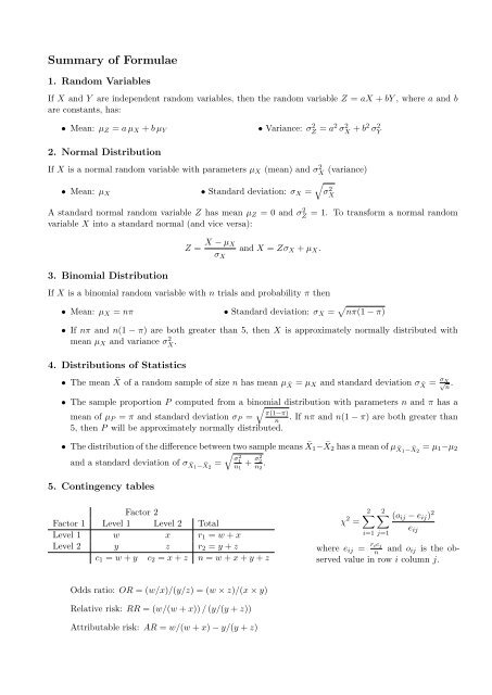
Summary of Formulae1. Random VariablesIf X and Y are independent random variables, then the random variable Z = aX + bY , where a and bare constants, has:• Mean: µ Z = a µ X + b µ Y• Variance: σ 2 Z = a2 σ 2 X + b2 σ 2 Y2. Normal DistributionIf X is a normal random variable with parameters µ X (mean) and σX 2 (variance)√• Mean: µ X • Standard deviation: σ X = σX2A standard normal random variable Z has mean µ Z = 0 and σZ 2variable X into a standard normal (and vice versa):= 1. To transform a normal randomZ = X − µ Xσ Xand X = Zσ X + µ X .3. Binomial DistributionIf X is a binomial random variable with n trials and probability π then• Mean: µ X = nπ • Standard deviation: σ X = √ nπ(1 − π)• If nπ and n(1 − π) are both greater than 5, then X is approximately normally distributed withmean µ X and variance σ 2 X .4. Distributions of Statistics• The mean ¯X of a random sample of size n has mean µ ¯X = µ X and standard deviation σ ¯X = σX √ n.• The sample proportion P computed from a binomial √ distribution with parameters n and π has aπ(1−π)mean of µ P = π and standard deviation σ P =n. If nπ and n(1 − π) are both greater than5, then P will be approximately normally distributed.• The distribution of the difference between two sample means ¯X 1 − ¯X 2 has a mean of µ ¯X1 − ¯X 2= µ 1 −µ 2and a standard deviation of σ ¯X1 − ¯X 2=√σ 21n 1+ σ2 2n 2.5. Contingency tablesFactor 2Factor 1 Level 1 Level 2 TotalLevel 1 w x r 1 = w + xLevel 2 y z r 2 = y + zc 1 = w + y c 2 = x + z n = w + x + y + z2∑ 2∑χ 2 (o ij − e ij ) 2=i=1 j=1e ijwhere e ij = r ic jnand o ij is the observedvalue in row i column j.Odds ratio: OR = (w/x)/(y/z) = (w × z)/(x × y)Relative risk: RR = (w/(w + x)) / (y/(y + z))Attributable risk: AR = w/(w + x) − y/(y + z)

6. Confidence IntervalsAll of the 100(1 − α)% confidence intervals calculated in this course are of the form:Estimate ± multiplier × standard error.In the following ¯x, p etc are the values calculated from the samples.Estimate df (ν) Multiplier Standard ErrorPopulation mean• Random sample, σ x known ¯x NA z α/2√σ Xn• Random sample, normal population,¯x n − 1 t α/2,ν√snσ xunknownDifference between population means• Small random samples, normal population,σ 1 = σ 2 = σ unknown¯x 1 − ¯x 2 n 1 + n 2 − 2 t α/2,ν√(n1 −1)s 2 1 +(n 2−1)s 2 2n 1 +n 2 −2• Large random samples (both ≥ 30) ¯x 1 − ¯x 2 NA z α/2√s 21• Paired difference in random samples ¯d n − 1 t α/2,νs dfrom a normal populationn 1+ s2 2n 2√n√1n 1+ 1 n 2Population proportions√p(1−p)• Population proportion p NA z α/2√ n• Difference between 2 population p 1 − p 2 NA zp1 (1−p 1 )α/2 n 1+ p 2(1−p 2 )n 2proportionsOdds ratio, relative risk, attributable risk (see contingency tables above for w, x, y and z)• Log (natural) odds ratio ln(OR) NA z α/2√1w + 1 x + 1 y + 1 z• Log (natural) relative risk ln(RR) NA z α/2√1w − 1w+x + 1 y − 1y+z• Attributable risk – as for the difference of two population proportionswith p 1 = w/(w + x) and p 2 = y/(y + z)After ANOVA and Regression• Estimate, multiplier and standard errors determined from output7. ANOVA1. MS = SS / df2. General SS = nȳ 23. Group SS = C2 1n 1+ C2 2n 28. Regressionŷ = ˆβ 0 + ˆβ 1 x where ˆβ 1 =where s e =√ ∑(yi−ŷ i ) 2n−2+ . . . + C2 kn k− nȳ 2 .∑ (xi −¯x)(y i −ȳ)∑ (xi −¯x) 2 and ˆβ 0 = ȳ− ˆβ 1¯x. Standard error of the slope SE( ˆβ 1 ) =√ s e ∑(xi , −¯x) 2= √ MS Residual. Standard error of a forecast at x k = s e√1 + 1 n + (x k−¯x) 2 ∑ (xi −¯x) 2 .