Course Notes - Department of Mathematics and Statistics

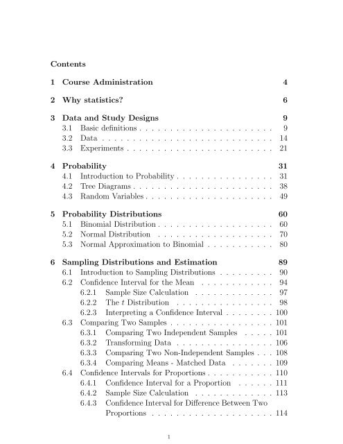
Contents1 Course Administration 42 Why statistics? 63 Data and Study Designs 93.1 Basic definitions . . . . . . . . . . . . . . . . . . . . . . 93.2 Data . . . . . . . . . . . . . . . . . . . . . . . . . . . . 143.3 Experiments . . . . . . . . . . . . . . . . . . . . . . . . 214 Probability 314.1 Introduction to Probability . . . . . . . . . . . . . . . . 314.2 Tree Diagrams . . . . . . . . . . . . . . . . . . . . . . . 384.3 Random Variables . . . . . . . . . . . . . . . . . . . . . 495 Probability Distributions 605.1 Binomial Distribution . . . . . . . . . . . . . . . . . . . 605.2 Normal Distribution . . . . . . . . . . . . . . . . . . . 705.3 Normal Approximation to Binomial . . . . . . . . . . . 806 Sampling Distributions and Estimation 896.1 Introduction to Sampling Distributions . . . . . . . . . 906.2 Confidence Interval for the Mean . . . . . . . . . . . . 946.2.1 Sample Size Calculation . . . . . . . . . . . . . 976.2.2 The t Distribution . . . . . . . . . . . . . . . . 986.2.3 Interpreting a Confidence Interval . . . . . . . . 1006.3 Comparing Two Samples . . . . . . . . . . . . . . . . . 1016.3.1 Comparing Two Independent Samples . . . . . 1016.3.2 Transforming Data . . . . . . . . . . . . . . . . 1066.3.3 Comparing Two Non-Independent Samples . . . 1086.3.4 Comparing Means - Matched Data . . . . . . . 1096.4 Confidence Intervals for Proportions . . . . . . . . . . . 1106.4.1 Confidence Interval for a Proportion . . . . . . 1116.4.2 Sample Size Calculation . . . . . . . . . . . . . 1136.4.3 Confidence Interval for Difference Between TwoProportions . . . . . . . . . . . . . . . . . . . . 1141

7 Hypothesis Testing 1197.1 Hypothesis Test for Mean . . . . . . . . . . . . . . . . 1217.2 Hypothesis Test For Proportion . . . . . . . . . . . . . 1227.3 Hypothesis Test Difference Two Means . . . . . . . . . 1237.4 Hypothesis Test Difference Two Proportions . . . . . . 1277.5 Interpreting the p-value . . . . . . . . . . . . . . . . . 1297.6 Significance and Conclusiveness . . . . . . . . . . . . . 1307.7 Power . . . . . . . . . . . . . . . . . . . . . . . . . . . 1338 Contingency Tables 1398.1 Introduction to Contingency Tables . . . . . . . . . . . 1408.2 Relative Risk (RR) . . . . . . . . . . . . . . . . . . . . 1438.3 Attributable Risk (AR) . . . . . . . . . . . . . . . . . . 1448.4 Odds Ratio (OR) . . . . . . . . . . . . . . . . . . . . . 1448.5 Confidence Intervals for Risk Measures. . . . . . . . . . 1468.6 Chi Square Test for Contingency Tables. . . . . . . . . 1538.6.1 Simpson’s Paradox . . . . . . . . . . . . . . . . 1588.6.2 Test for Trend . . . . . . . . . . . . . . . . . . . 1609 ANOVA 1669.1 One Factor ANOVA . . . . . . . . . . . . . . . . . . . 1679.1.1 The ANOVA Model . . . . . . . . . . . . . . . . 1699.1.2 Partitioning the Sum of Squares . . . . . . . . . 1699.1.3 F Distribution . . . . . . . . . . . . . . . . . . . 1719.1.4 Computational Formulae . . . . . . . . . . . . . 1719.2 Post ANOVA Analysis . . . . . . . . . . . . . . . . . . 1749.2.1 CI for the Mean . . . . . . . . . . . . . . . . . . 1769.2.2 CI for the Difference Between Two Means . . . 1779.2.3 Multiple Comparisons . . . . . . . . . . . . . . 1789.3 ANOVA Assumptions . . . . . . . . . . . . . . . . . . . 1789.4 Two factor ANOVA . . . . . . . . . . . . . . . . . . . . 1799.4.1 Block Designs . . . . . . . . . . . . . . . . . . . 1839.5 Two Factor Factorial Experiments . . . . . . . . . . . . 1869.5.1 Interpreting the Interaction Effect . . . . . . . . 1912

10 Regression 20210.1 Introduction to Regression . . . . . . . . . . . . . . . . 20310.2 Checking fit of Regression . . . . . . . . . . . . . . . . 21210.3 Confidence Intervals and Regression . . . . . . . . . . . 21810.4 Correlation . . . . . . . . . . . . . . . . . . . . . . . . 22310.5 Multiple regression . . . . . . . . . . . . . . . . . . . . 23010.6 Are all the variables required? . . . . . . . . . . . . . . 23810.7 Analysis of Covariance . . . . . . . . . . . . . . . . . . 24510.8 Logistic Regression . . . . . . . . . . . . . . . . . . . . 253A Tools for assignments 267B Summary of Formulae 2713

1 Course AdministrationAdministration• Lectures: Monday, Tuesday, Wednesday, Thursday ∗ at 8am or10am• Tutorials will be cafeteria style, students are free to attend atany scheduled tutorial time. Tutorials are held in the North CAL(computer laboratory, opposite entrance to the Science Library inthe Science III building)..• Tutorials will be held 9am to 3pm Tuesday through Thursday4

Resource PageDepartment of Mathematics and Statistics (http://www.maths.otago.ac.nz)• Download course information• Access and submit assignments and mastery tests (assignmentsavailable from 9am Mondays)• Book slots for mastery tests• View assignment/test results• Questionnaire - please fill out (voluntary)Assessment• Internal assessment will count for 1/3 of your final mark withplussage (your internal assessment counts only if it helps i.e. wewill take the better of your final mark or 1/3 internal + 2/3 final).• Internal component is made up of two parts:- 1/3 from assignments, 8 in total (due Friday 9am in semesterweeks 2-4, 6-7 and 9-11)- 2/3 from short mastery tests, 3 in total (in semester weeks 5,8 and 12)Assignments/Tests• All on-line• Assignments can be submitted from anywhere in the world• You will need access to R- Free software which you can download5

- CAL labs- Halls of Residence• Tests are only administered in North CALPolicy on collaboration• Tests and assignment questions are individualised• There may be some questions requiring written answers• On assignments (but not tests) we are happy for students to discussanswers. However,• We insist that you answer questions in your own words.- Our software checks students answers against the entire class2 Why statistics?Why do we study statistics?• Statistics refers to both data and to the theory and logic supportingthe toolkit of techniques we use to study data.• The main reason students study ‘Statistics’ is because they areforced to...• We are curious and we collect data in order to understand betterthe world around us- the persuasive power of numbers• Published numbers have a power they often don’t deserve.- if a statistic seems unbelievable, don’t believe it• Research and management (policy).6

3 Data and Study Designs3.1 Basic definitionsDefinitions• Each question has a numerical answer (counts, probabilities, proportions,...).• Need a toolkit for numerical description and for answering numericalquestions.• Inference – formal name given to learning from data using statisticaltools.• We need some agreed terminology.Population• Population Complete set of entities or elements or units or subjectsthat we wish to describe or make inference about. Real orhypothetical.Well-defined- The collection of words in poems by W. B. Yeats.- All the rimu trees in Tongariro National Park.Not well-defined- The population of New Zealand. Right now? Past? Future?- Banks Peninsula Hector’s dolphins. Which dolphins shouldwe include?- Target population in a drug trial. All alive or who will ever beborn? Over a certain age? Only those people who can affordthe drug?Which population have we studied? Which are we interested in?9

Sample• A Sample is a subset of a population.A ‘census’ is a complete enumeration/sample of a population.Rare.Samples need to be ‘representative’. Only guaranteed by randomselection.What if random sampling is impossible?- We have to assume that our sample is representative.- Not testable and dangerous. Faith in our procedure.10

Parameter• Parameter: Fixed number that characterises a population.- The number of people alive in NZ at midnight on 1/1/2000.- The average height of all 2013 STAT110 students.Parameters are either known or unknown, hypothetical, or real.Much of statistics is about obtaining intelligent guesses for parameters.Usually represented by a Greek letter: α, β, γ, δ, . . ..Hypothetical?• Does the parameter really exists?WomenMenTime140 160 180 200●●Asymptote = 2hr 14min 51sec●●● ●● ●●●●●●●● ● ●● ● ●● ●●●Time130 140 150 160 170●●●●●Asymptote = 1hr 58min 48sec●●●●●●● ●●●● ●●●● ● ●●●●●●●●●1970 1980 1990 20001920 1960 2000YearYearRandom variable• Random variable Mathematically precise definition not reallyhelpful.11

2h 15:25 (2003)2h 03:38 (2011)- An unknown quantity that varies in an unpredictable way.- Once observed we refer to a realised value.12

TypesDiscrete - can put in one-to-one correspondence with the countingnumbers.Continuous - can be expressed on a continuous scale in whichevery value is possible.Categorical - restricted to one of a set of categories. For example‘Heads’ or ‘Tails’.Random variables notationNotation Represented by upper case Roman lettersLower case Roman letter represents the observed value.Pr(X = x) means ‘the probability that the random variableX takes the value x.e.g., Pr(X = 1.2).Random variables described by probability distributions.Observed values of random variables are data.Statistic• A statistic is a numerical summary of data.• An estimate is a special kind of statistic used as an intelligentguess for a parameter.- Usually denote an estimate by a circumflex: ˆµ is an estimateof µ.- Remember ˆµ is statistic and an estimate, µ is a parameter.Model• A model is a mathematical description of the data generatingmechanism.- Expressed in terms of parameters and random variables.13

• Think of it as a metaphor - if we repeatedly toss a coin we findthe sequence of ‘heads’ and ‘tails’ behaves in the same way as asequence of independent samples from a Bernoulli distribution.- Outcomes of coin tosses are data.- A Bernoulli distribution exists in theory only.3.2 DataData and inference• Proper inference depends on how our data were collected.• “In 20 tosses of a coin I obtained 20 heads”• But I tossed it 45 times.EarthquakesSouthern end of the alpine fault. Source: Te Ara - the Encyclopedia of New Zealand• Ruptured 1230, 1460, 1615 and 171714

- How do geologists know?- Sediment disturbances, radiocarbon dating of disturbed material,tree rings.• Intervals: 230, 155, 102, ≥ 293 years.- Overdue?Earthquake II• Observational – obtained by recording natural events.- Could the measurement have favoured the observed values?• Synthetic – reconstructed from other data.- Not the data we wish we had.- Reconstruction introduces error (1717 accurate to nearest year;before 1717 accurate to ± 50 years)• Last interval is censored – it is at least 293 years.• Need to take into account when expressing uncertainties associatedwith any predictions.15

Major sources of data• Sample surveys - study subjects selected through random sampling.- Probability samples and non-probability samples- Do not trust results from non-probability samples (judgmentsampling, snowball sampling, quota sampling, convenience sampling)- Examples: Questionnaires, quadrat sampling etc• Experiments - deliberate manipulation of variables to see response.- Replication, randomisation and control.- Sometimes one (or more) element is missing - quasi-experiments.• Observational studies - descriptive or quasi-experimental- If descriptive, probability sampling should be used for reliableinference.- If experimental, absence of randomisation implies weaker inference.Sample surveys• Inefficient (usually) to try and sample whole population- Usually impossible - even with a ‘census’• Which items do we include?- Need to guard against introducing bias.• Even with random sampling have to be watch out for nonresponsebias.16

Source: skyscrapercity.comSampling frame• Sampling frame - List of items in a population from which asample is drawn.• Rarely coincides with the entire population of interest.- Telephone numbers- Electoral roll- lists of licence holders• Often don’t exist- List of all Hector’s dolphins in New Zealand?- List of all potential buyers of a new drug• Even without a list we can ensure an unbiased sample if everyindividual has the same chance of being drawn.Example 1: Gamebird surveys• Gamebird hunting licence required – natural sampling frame.• Questionnaires used to estimate gamebird harvest in the 1980s.• Mailout plus one reminder then a telephone sample of randomlyselected nonrespondents.17

Gamebird survey results4 May 25 May 15 Jun 29 JunEstimate SE Estimate SE Estimate SE Estimate SEMallards harvestedR 6.17 0.58 4.36 0.67 2.80 0.51 2.38 0.41N 5.23 0.75 4.02 0.62 1.74 0.44 1.24 0.34Hours huntedR 9.67 0.57 8.18 1.16 5.43 0.76 4.91 0.65N 6.85 0.59 5.66 0.81 3.16 0.61 1.71 0.34Harvest by respondents (R) and non-respondents (N) to gamebird hunting questionnaire.Example 2: 1936 Presidential election• Literary Digest predicted 2:1 victory to Landon (R) over Roosevelt(D).• Election: Landon 2 states Roosevelt 46!• Mailout to more than 10 million – 2 million responded• Frame: readers of Literary Digest, telephone numbers, registeredcar owners.• George Gallup used a quota sample of 50,000 people to (a) predicta win for Roosevelt and (b) used a sample of 3000 from theLiterary Digest frame to predict that Literary Digest would mispredict.Probability sampling• We want our frame to match the population of interest and a wayto draw a representative sample.• Probability sampling is the only way to ensure representativeness• Simple random sample For a finite population of size N drawa sample of size n such that each possible sample has the sameprobability.- Lotto - each draw of 6 balls has the same probability18

- 1 in 3.8 million - 3.8 million distinct sequences, all equallylikely.- Sampling without replacementSimple random sample• Easy to analyse• let y 1 , . . . , y n denote the observed valuesEstimate population mean:∑ ni=1ˆµ = ȳ =y i.n‘add the values up and divide by their number’.Estimate population total:ˆT = N nn∑y i = Nȳ.‘take the sample mean and multiply by the population size.’i=1Stratified sampling• Much of statistical design theory is about controlling variation.• More variable data means less precise inference (signal vs noise).• Stratified sampling useful when the population comprises differenttypes of similar individuals.- A stratum is a population sub-division of similar units• Take a simple random sample from within each stratum.- More precise for the same expenditure.- Might be interested in the results by stratum.• Can take different sized samples from different strata.- Device for reducing the overall variability.• Formulae for estimates more complicated.- Consult an expert.19

Replication and randomisation• Replication Responses vary among subjects. Replication allowsus to separate out treatment effects from chance effects.• Randomisation Ensures that effects of unmeasured factors areequalised across the treatment groups.Control• Provides context for evaluating the effect of interest.• Often a placebo - determine existence of an effect• Sometimes a standard treatment – differences relative to the standard.- Effect of surgical sterilization on possum populations - shamsurgery.- Effect of lactate buffers on 800m time to exhaustion at 20kmph- salt tablets.- Growth and survival of starved paua larvae - no starvation.22

Important designs• Completely randomised designExperimental units allocated to treatment groups randomly.- No restriction on the allocations apart from the numbers ineach group.- Each possible allocation has the same probability of beingselected.• Randomised block designRandom allocation of treatments within blocks of similar subjects.- Reduces unexplained error by removing between-block variationBlock what you can, randomize what you cannot.Repeated measures• Individuals can act as their own blocks• Each individual receives each treatment, usually in a differentorder- Effect of lactate buffers on time to exhaustion at 20kmh- Each subject received each of the 4 treatments in randomorder.• Paired t-test special case of analysis when just two treatments(eg, treatment and control)- Need special care where the order of treatment matters (e.g.,learning)23

Polio vaccine trial• Acute viral disease spread by person-to-person contactPolio cases (deaths in red) in NZCases0 200 400 600 800 1000 12001920 1940 1960 1980 2000YearPolio vaccine trial• Mass vaccination of children in NZ in 1961 and 1962• Followed US trials involving 1.8M children- Trial needed because of earlier failures- Massive size needed because of low prevalence• Controversy over the design – parental consent required and soonly studying volunteers.Polio vaccine trial II• Two designs usedA. Observed control - 1st and 3rd graders acted as controls and2nd graders with parental consent vaccinated.24

B. Randomised control - of all children who had parental consent,half were randomly allocated to the control group and theother half vaccinated.- The control group were “vaccinated” with a saline solution- Children, Drs, researchers didn’t know which child was inwhich group until after the experiment.Polio vaccine trial IIIDesign Trt group n Cases Rate (per 100,000)Observed Control Vaccinated 221998 56 25.2Observed Control Controls 725173 391 53.9Randomised Control Vaccinated 200745 57 28.4Randomised Control Placebo 201229 142 70.6• Observed control design biased against the vaccine.- Confounding of vaccine effect and ‘parental consent’ effect.- Children from poorer families had a natural level of immunityand less likely to receive consent for involvement in the trial.Chance effect or real?• Just by chance things almost always differ. Could this be chance?• Suppose we have two unfair coins, a ‘Control’ coin and a ‘Vaccine’coin• We toss the control coin 201,229 times and the other one 200,645times.• If they had the same chance of coming up heads what is theprobability of observing the outcome 142 heads for the controlcoin and 57 for the vaccine coin, or a more extreme one?- More than one billion to one against- Coins are not the same.25

Confounding• Between 1972 and 1974 1/6 of women on electoral roll of Whickhamsurveyed.• Followed up 20 years laterSmokerYes No TotalDead 139 230 369Alive 443 502 945582 732 1314Smokers Death rate = 139/582 or 23.9%.Non-smokers Death rate = 230/732 or 31.41%.• Statistics don’t lie!Simpson’s paradoxAgeSmoking status 18-24 25-34 35-44 45-54 54-64 65-74 75+Smoker 3.6 2.4 12.8 20.8 44.3 80.6 100Non-smoker 1.6 3.2 5.8 15.4 33.1 78.3 100Proportion dead by the time of the follow up survey.• Death rate is higher for smokers in every age group except one!• Few of the older women (65+) were smokers at the time of theoriginal survey but most had died by the time of follow-up.• Smokers had already disappeared from these age groups at thetime of the initial survey.Dealing with confounders• In experiments we randomize to equalize all other effects acrossour treatment groups.• In observational studies we must measure potential confounders- Always a risk that we have missed confounders26

- Reason why observational studies provide a weaker form ofevidence.• Confounding can be usefulDeliberate confounding• STAT110 questionnaire - last question• We deliberately confounded response with coin toss to provideanonymity• Out of 267 responses, 108 tails and 159 heads- We expect ∼ 133.5 tails- 133.5-108 = 25.5 is our guess for the number of missing ’tails’reported as ’heads’ because of drug use.• 25.5/133.5 = 0.191 - guess that approx. 19.1% of the class havetried drugs (22.6% last year)..• Good model for the confounding (coin toss) - can undo the confounding.Cohort Studies• Whickham smoking study is a cohort study- longitudinal- prospective - outcome of interest becomes manifest over time- observational - alternative to experiment when these are impossible• Famous local example: Dunedin Multidisciplinary Health and Developmentstudy- Cohort study of 1,037 people born in Dunedin in 1972/1973- Follow up: 3,5,7,9,11,13,15,18,21,26, and 32; 38 underway.• Cohort studies may also look backward in time (retrospective)27

Case-Control Study• Retrospective• Doll-Hill study of British cancer patients (1948-1952).- Cases = lung cancer- Controls = other forms of cancer, matched to the cases by ageand sex.Cases ControlsSmokers 1350 1296Nonsmokers 7 61Total 1357 1357• Nonsmokers 7/1357 = 0.51% of the male cases but 61/1357 =4.5% of the male controls• Implicates smoking as a factorTrout Cod• Case-control studies commonly associated with epidemiology• Can be applied usefully in other settings• Habitat selection of trout cod on the Murray River- Cases = locations where radio-tagged trout cod were found- Controls = randomly selected locations28

Things that go wrong• Even the best studies strike problems• Missing data- Survey nonresponse- Recording error- Treatments may fail- Study plots may be destroyed (demonic intrusion)Why are the data missing?• Should always ask why the data are missing• If the ‘missingness mechanism’ is related to the response of interestthen may cause bias- e.g., Non-response bias- ‘Non-ignorable’ missingness requires specialised help• Censoring is a special case- Right-censoring - true value is larger than the recorded value- Left-censoring - true value is smaller than the recorded value- Interval-censored - true value lies between 2 known values• In survival studies longer-lived individuals more likely to be rightcensored29

Good and Bad studies• Reliable samples and surveys will:1. Employ formal probability-based sampling when selecting individualsto sample.2. Employ well-constructed sampling frames, and these shouldinclude the entire population of interest or nearly so.• Reliable experiments will3. Randomly allocate treatments to subjects to avoid confoundingand employ a control.4. Use blocking to remove unwanted sources of variation.5. Select study units that represent the population of interest.This should be done using random selection.Compromise• Compromise is often unavoidable- Randomisation of treatments may be impossible ethically- It may be impossible to sample individuals randomly.• Don’t substitute ‘difficult’ for impossible- A smaller number of well-designed studies is better than awhole lot of cheap ones.• Watch out for designs that cheat.30

4 ProbabilityFred’s DayFred awoke one morning and headed off to the doctor. In the waitingroom for the doctor the 23 waiting paitents were asked their birthdays.Fred could not help but overhear that two of the patients were born onthe same day, it was not his birthday though. During his appointmentFred got tested for a rare disease (1 in 10000 people suffer this disease),the test returns a positive result in 95% of cases of people who actuallyhave the disease, and 6% of cases when people don’t have the disease.Fred’s doctor informed him that he had returned a positive result.Should Fred be worried about returning a positive test result? Whatis the likelihood he has the disease?What is the probability of 2 out of 23 people in a room sharing abirthday? What are the odds that they share a specific birthday?In the next section we will learn some skills that will help us answerthese questions.4.1 Introduction to ProbabilityI have data now what?• Now we have learnt about collecting data, we want to know whatwe can do with itFirst of all: What is Probability?• There is no consistent definition of probability• Statisticians can be split into two main groups who have differingviews on probability.• Frequentists consider probability to be the relative frequency ‘inthe long run’ of outcomes.31

• Bayesians consider probability to be a way to represent an individual’sdegree of belief in a statement given the evidence.• Consider these statements.• We can quantify these probabilities.What is the probability I win lotto tonight?What is the probability I roll a 6.• Based on personal and subjective beliefWhat is the probability I pass Stat110?What is probability I will do an OE after graduating?Some definitions• Experiment = process by which observations/measurements areobtained e.g. tossing a fair die• Event = outcome of experiment e.g. getting a 6• Sample space = set of all possible outcomes e.g. 1, 2, 3, 4, 5, 6Conditions for a valid probability1. Each probability is between 0 and 12. The sum of the probabilities over all possible simple events is 1.In other words, the total probability for all possible outcomes ofa random circumstance is equal to 1. (As long as these events aremutually exclusive)What does probability mean?• If the event A cannot happen then Pr(A) = 0• If the event A is certain to happen then Pr(A) = 1• Let’s say we have a mouse trap.• The event that the mouse we trap is a male and pregnant has aprobability Pr(A) = 0 of occuring because this is impossible32

• The event that the mouse we trap is either male or female hasa probability Pr(A) = 1 of occuring because it will definitely beone or the other.Calculating Probabilities• Probability of an event A isPr(A) =no. of experiments resulting in Alarge no. of repetitions= n AN• We don’t always need to conduct the experiments as we can makesensible assumptions i.e. die or coin is fair (prob of each outcome= 1/6 or 1/2 respectively)Some more things to knowComplementary Events• Two events are complementary if all outcomes are either of thetwo events e.g head or tail on fair coin• Ā is called the complement of A.Pr(A) + Pr(Ā) = 1The RulesAddition RulePr(A or B) = Pr(A ∪ B) = Pr(A) + Pr(B) − Pr(A ∩ B)Multiplication RulePr(A and B) = Pr(A ∩ B) = Pr(A) Pr(B|A)Addition rule - special caseMutually Exclusive Events• There is no intersection between the two events. In lay termsevents are said to be mutually exclusive if they cannot occur togetheri.e. getting heads and tails33

• In this case the addition rule simplifies toPr(A or B) = Pr(A ∪ B) = Pr(A) + Pr(B)• Because Pr(A ∩ B) cannot occurMultiplication rule - special caseIndependent Events• When the occurence of one event does not effect the outcome ofanother event. i.e. getting 3 heads in a row• In this case the multiplication rule simplifies toPr(A and B) = Pr(A ∩ B) = Pr(A) Pr(B)• Because Pr(B|A) = Pr(B), since B no longer relys on A happening.Blood donor example• The probability of being in each of the 4 blood groups (Dunedindonor centre)Blood Type ProbabilityA 0.38B 0.11AB 0.04O 0.47Blood donor example - Addition Rule• What is the probability that a person is either A or B?Pr(A or B) = Pr(A) + Pr(B)= 0.38 + 0.11= 0.4934

Blood donor example - Multiplication RuleWhat is the probability that 3 randomly selected people have bloodgroup O?Pr(O) × Pr(O) × Pr(O) = 0.47 3= 0.104(under the assumption independence)Hospital Patients• A survey of hospital patients shows that the probability a patienthas high blood pressure given he/she is diabetic is 0.85. If 10%of the patients are diabetic and 25% have high blood pressure:• Find the probability a patient has both diabetes and high bloodpressure.• Are the conditions of diabetes and high blood pressure independent?Hospital Patients - Relevant information• Let A be the event ‘A patient has high blood pressure’• Let B be the event ‘A patient is diabetic”• Pr(A|B) = 0.85• Pr(B) = 0.10• Pr(A) = 0.25Hospital Patients - Question 1• Find the probability a patient has both diabetes and high bloodpressure.Pr(A ∩ B) = Pr(A | B) × Pr(B)= 0.85 × 0.10= 0.08535

Hospital Patients - Question 2• Are the conditions of diabetes and high blood pressure independent?• Remember when discussing the special case of the multiplicationrule we said if A and B are independent then:Pr(A | B) = P r(A)• We can use this to test for independence.Pr(A | B) = 0.85Pr(A) = 0.25Pr(A) ≠ Pr(A | B)• ∴ A and B are not independentCalculating Conditional probabilities• Conditional Events• Two events are conditional if the probability of one event changesdepending on the outcome of another event e.g EXAMPLEPr(A ∩ B) = Pr(A) Pr(B | A)Pr(A ∩ B) ÷ Pr(A) = Pr(A) Pr(B | A) ÷ Pr(A)P r(A ∩ B)Pr(B | A) =Pr(A)Pr(B | A) =P r(A ∩ B)Pr(A)• Important not to interpret conditional results as unconditional• What is the probability of buying ice cream?• Hot day = High, Cold day = Low36

Fair Die Example• A fair die is thrown. A is the event ’a number greater than 3 isthrown’ and B is the event ’an even number is thrown’• Find Pr(A ∪ B) and Pr(A ∩ B)Pr(A) =3/6 = 1/2 Pr(B) =3/6 = 1/2Fair Die Example - Visualisation• A fair die is thrown. A is the event ‘a number greater than 3 isthrown’ and B is the event ‘an even number is thrown’524613Pr(A ∪ B) = (2 4 5 6)Pr(A ∩ B) = (4 6)Fair Die Example• Find Pr(A ∩ B)• Use multiplication rule, because events are not independent :• We can find the conditional probability of Pr(B | A)Pr(A ∩ B)Pr(B | A) =Pr(A)P r(B | A) = 1/31/2P r(B | A) = 2/337

• Or we can calculate P r(A ∩ B)Pr(A ∩ B) = Pr(A) Pr(B | A)Pr(A ∩ B) = 1/2 × 2/3Pr(A ∩ B) = 1/3• The decision on which to calculate depends on the informationwe have.• Find P r(A ∪ B)• Use addition rule, because events are not mutually exclusivePr(A ∪ B) = Pr(A) + Pr(B) − Pr(A ∩ B)Pr(A ∪ B) = 1/2 + 1/2 − 1/3Pr(A ∪ B) = 2/34.2 Tree DiagramsTree Diagrams• Useful for helping calculate the probability of a combined event• The stages of the combined event can be independent or dependent• A dependent stage means the probability at each branch is conditionalon earlier outcomes.• Tree diagrams show all possible outcomes38

Tree diagram rules• Add Vertically.• Multiply across.• They give a good way to visualise sample space restrictions resultingfrom conditioning and help to calculate joint and conditionalprobabilitiesBasic Tree DiagramsBA¯BBĀ¯B• In this simple example each of the levels of the tree diagram havetwo possibilities.• Note A + Ā = 1 and B + ¯B = 1. Since if A does not occur Āmust, similarly if B does not occur ¯B must.• Also note if the events A and B are not independant than theprobability B occurs after A is not necessarily the same as theprobability B occurs after Ā39

Handedness vs Gender - Combined Probabilities0.5696F0.89140.1086R 0.5077L 0.06190.4304M0.8897R 0.38290.1102L 0.0474Handedness Summary• What is the probability of each of being Left handed?Pr(L) = Pr(L ∩ F ) + Pr(L ∩ M)Pr(L) = 0.0619 + 0.0474Pr(L) = 0.1093• What is the probability of each of being right handed?Pr(R) = Pr(R ∩ F ) + Pr(R ∩ M)Pr(R) = 0.5077 + 0.3829Pr(R) = 0.8906Independent Stages• Stephens Island is an uninhabited island in Cook Strait wheretuatara are being re-established. For some years three locationshave been visited on the island and tuatara have been found ata location with probability 0.4. At any visit X represents thenumber of locations out of three at which tuatara are observed.X can take values 0, 1, 2, or 3. Find the probabilities that 0, 1,2, or 3 locations have tuatara on a visit. T is the event ‘locationhas tuatara’ and N is the complementary event ‘location has notuatara’40

Tree Diagrams - Independent Stages0.60.4TN0.40.60.40.6TNTN0.40.60.40.60.40.60.40.6T X = 3N X = 2T X = 2N X = 1T X = 2N X = 1T X = 1N X = 0Independent Stages• Find the probability of seeing tuatara at two of the three sites:P r(X = 2) = P r(TTN, TNT, NTT)= 0.4 × 0.4 × 0.6 +0.4 × 0.6 × 0.4 +0.6 × 0.4 × 0.4= 0.096 + 0.096 + 0.096= 0.288• Find the probability of seeing tuatara at one of the three sites• Take advantage of the fact that all possibilities add to 1P r(X = 2) = 0.288P r(X = 0) = 0.6 × 0.6 × 0.6 = 0.216P r(X = 3) = 0.4 × 0.4 × 0.4 = 0.06441

P r(X = 1) = 1 − 0.288 − 0.216 − 0.064= 0.43242

Dependent Stages• Andrew, John and Mark play a game of chicken. There are sixsimilar cars, two of which have had the brakes disabled. Eachperson chooses a car at random, drives at high speed towards ariver, and brakes in time to stop. The boys decide to proceed inalphabetical order• Find Pr(each will lose) and Pr(no loser) where the game stopswhen the first boy drives into the river.2/6Andrew LosesJohn Loses4/63/52/52/4Mark Loses2/4No loserPr(Andrew loses) = 2/6= 1/3Pr(John loses) = 4/6 × 2/5= 4/15Pr(Mark loses) = 4/6 × 3/5 × 2/4= 3/15Pr(no loser) = 4/6 × 3/5 × 2/4= 1/5DefinitionsSensitivity = Pr(B| A) The probability that a person with thedisease returns a positive result.Specificity = Pr(¯B| Ā) The probability that a person withoutthe disease returns a negative result.43

Definitions IIPositive Predictive Value = Pr(A|B) The proportion of patientswith positive test results who are correctly diagnosed.Negative Predictive Value = Pr(Ā|¯B) The proportion of patientswith negative test results who are correctly diagnosed.Screening Programmes• A patient with certain symptoms consuled her doctor to be checkedfor a cancer, and she undergoes a biopsy.• With this test there is a probability of 0.90 that a woman withthe cancer shows a positive biopsy, and a probability of only 0.001that a healthy woman incorrectly shows a positive biopsy.• Historical information also suggests that the prevalence of thiscancer in the population is 1 in 10000.• Find the probability that a woman has the cancer given the biopsysays she does (i.e. does the biopsy diagnose true patient status?).• Let A be the event ‘woman has the cancer’ and B be the event‘biopsy is positive’.• Pr(A) = 1/10000 = 0.0001 (disease prevalence)• Pr(B| A) = 0.90 (conditional probability)• Pr(B| Ā)= 0.001 44

0.90BBiopsy +ve (true positive)0.00009A0.00010.10¯BBiopsy -ve (false negative)0.000010.99990.001BBiopsy +ve (false positive)0.00100Ā0.999¯BBiopsy -ve (true negative)0.99890Probability that the test is +ve = 0.00009 + 0.00100 = 0.00109Positive Predictive value• Find the positive predictive value Pr(A|B). To calculate this weuse the conditional probability formulaP r(A ∩ B)P r(A| B) =P r(B)P r(Have disease and test positive)P r(A| B) =P r(test positive)P r(True positive)P r(A| B) =P r(Total positive)P r(A| B) = 0.000090.00109P r(A| B) = 0.083• Only 8.3% of those women identified as having the disease actuallydo.45

Negative Predictive value• Find the positive predictive value Pr(A|B). To calculate this weuse the conditional probability formulaP r(Ā| ¯B) P r(Ā ∩ ¯B)=P r(¯B)P r(Ā| ¯B) P r(Don’t have disease and test negative)=P r(test negative)P r(Ā| ¯B) P r(True negative)=P r(Total negative)P r(Ā| ¯B) = 0.998900.99891P r(Ā| ¯B) = 0.9999• 99.99% of those women identified as not having the disease actuallydo.Classification table• Sometimes the information is presented in a different manner.• Hooker Sealions• Closure of the squid fishery in the sub Antartic islands due toHooker sea lion bycatch is a costly issue for fishing companiesand much research is carried out on this. The following tableclassifies a sample of 219 vessels according to vessel nation andbycatch status over nine years.NZ Russia TotalNo by-catch 90 100 190Bycatch 6 23 29Total 96 123 219• Estimate the probability that a sampled vessel is Russian.• Given that the sampled vessel had by-catch what is the probabilitythat it is Russian.• Let B be By-catch, and ¯B be no-bycatch46

Calculating Probabilities• Estimate the probability that a sampled vessel is Russian.• The estimated probability a sampled vessel is Russian is 123219 =0.562Tree Diagram23123B23219R123219100123¯B10021996219696B6219NZ9096¯B90219Calculating Conditional Probabilities• Given that the sampled vessel had by-catch what is the probabilitythat it is Russian.• First calculate the total probability of a by-catchPr(B) = 23219 + 6219Pr(B) = 29219• Now use the conditional probabilityPr(R ∩ B)Pr(R | B) =Pr(B)Pr(R | B) =2321929219Pr(R | B) = 2329Pr(R | B) = 0.79347

Sensitive Survey Questions• Sometimes we are interested in sensitive survey questions.• For example the drug question in the questionaire.• The reason the question was phrased like this is it protects theindividual respondents.• If you got “heads” OR if you have ever smoked marijuana or usedany other illicit drug select “head”, otherwise select “tails”.Tree DiagramH0.50.51 - θTTθH (drugs)Sensitive Survey Question• So we can use this information to calculate probability of Druguse.P r(H) = P r(H) + P r(H(Drugs))P r(H) = 0.5 + (0.5 × (θ))• From the survey we got Pr(H) = 187305 = 0.61310.6131 = 0.5 + (0.5 × (θ))0.6131 − 0.5 = 0.5 + (0.5 × (θ)) − 0.50.1131 × 2 = (0.5 × (θ)) × 20.2262 = θ48

4.3 Random VariablesRandom Variables• A random variable has values which depend on the outcome of arandom experiment.• Random variables are labelled with a capital letter.• They can be discrete or continuousRandom Variables - Discrete Example• Consider the Tuatara example• The three previous locations are visited on 50 occasions and thenumber of locations with tuatara found are recorded each time.fX = x i f i i nPr(X = x i )0 8 0.16 0.2161 22 0.44 0.4322 15 0.30 0.2883 5 0.10 0.064Total 50 1.00 1.000• X is the random variable• X is discrete• The 50 responses are summarised as relative frequencies.• If many trials are carried out then the relative frequencies of eachx i ’s stabilise to give the probabilities for each outcome.• This set of probabilities forms the probability distribution49

Probability DistributionNote that for a probability distribution:• The sum of all the probabilities Pr(X = x i ) adds to one (same asfor relative frequency distribution).4∑Pr(X = x i ) = 1i=1• All probabilites are between 0 and 1.Describing Probability Distributions• Just as for a data set, we can describe a probability distributionby finding the mean (to describe the centre) and by finding thevariance or standard deviation (to describe the variability).If X is the probability distribution then:• µ X is the mean of X, and• σ 2 Xis the variance of XCalculating the Mean• For a sample of n values from the distribution, each x i occurs f itimes and there k possible values of i.• The sample mean is:¯x ==k∑x i f ii=1nk∑ f ix ini=1µ x =k∑x i Pr (X = x i )i=150

Calculating the Variance• The sample variance is:σ 2 x =k∑(x i − µ x ) 2 Pr (X = x i )i=1Finding the mean• Consider the Tuatara exampleX = x i Pr(X = x i ) x i Pr(X = x i )0 0.216 01 0.432 0.4322 0.288 0.5763 0.064 0.192Total 1.000 1.2• The mean number tuatara we see on each visit is 1.2Finding the variance• Consider the Tuatara exampleX = x i Pr(X = x i ) (x i − µ X ) 2 (x i − µ X ) 2 Pr(X = x i )0 0.216 (0 − 1.2) 2 = 1.44 0.3111 0.432 (1 − 1.2) 2 = 0.04 0.0172 0.288 (2 − 1.2) 2 = 0.64 0.1843 0.064 (3 − 1.2) 2 = 3.24 0.207Total 1.000 5.36 0.72• Variance is 0.72• Standard deviation is just the square root of the variance, hencethe s.d. = √ 0.72 = 0.85Contagious disease• A person infected with a disease can pass it on to others• Let the random variable X be the number of others infected bythis person.This time instead of setting up the table, lets just use the formula:51

X = x i Pr(X = x i )0 0.101 0.252 0.403 0.204 0.05Meanµ X = 0(0.10) + 1(0.25) + 2(0.40) + 3(0.20) + 4(0.05) = 1.85Varianceσ 2 X = (0 − 1.85)2 × 0.10 + (1 − 1.85) 2 × 0.25 + (2 − 1.85) 2 ×0.40 + (3 − 1.85) 2 × 0.20 + (4 − 1.85) 2 × 0.05 = 1.0275Standard Deviationσ X =√σ 2 X = √ 1.0275 = 1.0137Combining Random Variables• Often we are interested in the mean and the variance of a rescaledrandom variable, or in the mean and variance of sums (or differences)of random variables.• We will look at some properties of random variables (both discreteand continuous)Modifying Random Variables• If X is an independent random variable and a and b are constants.• Consider a new random variable Y, where:Y = a + bX• The mean of Y can be calculated by:µ Y = a + bµ X• The variance of Y can be calculated by:σY 2 = b2 σX252

Examples• Consider a data set XX = 3, 4, 5, 6, 7• So µ X = 5 and σX 2 = 2.5• Now consider Y = 2 × XX = 6, 8, 10, 12, 14• In this case a = 0 and b = 2 soµ Y = a + bµ X = 0 + 2 × 5 = 10σY 2 = b2 σX 2 = 22 × 2.5 = 10• So µ X = 5 and σX 2 = 2.5• Now consider Y = 4 × X + 3X = 15, 19, 23, 27, 31• In this case a = 3 and b = 4 soµ Y = a + bµ X = 3 + 4 × 5 = 23σY 2 = b2 σX 2 = 42 × 2.5 = 40Temperature Problem• Temperatures can be recorded in degrees Fahrenheit. Suppose arandom variable F measures January temperature ( ◦ F) in Dunedin.• Daily maximum summer temperatures have a mean of 70 ◦ F witha standard deviation of 5 ◦ F.• Use the conversion formula C = 5 9(F-32) to find the mean andstandard deviation for the temperature in degrees Celsius.53

Rearranging the FormulaC = 5 (F − 32)9= 5 ( ) 59 F − 9 × 32= 5 9 F − 1609= − 1609 + 5 9 FCalculating the mean• So to find µ C = µ a+bF , a = − 1609and b = 5 9µ C = a + bµ F= − 1609 + ( 59 × 70 )= 21.1 ◦ CCalculating the standard deviation• So to find σ 2 C = σ2 a+bF , a = −160 9and b = 5 9σC 2 = b2 σF2( ) 2 5= × 5 29= 7.716 ◦ C• The Standard deviation is just the square root of the variance√7.716 = 2.78 ◦ C54

Combining 2 Random Variables• If X and Y are an independent random variables and a and b areconstants.• Consider a new random variable Z, where:Z = aX + bY• The mean of Z can be calculated by:µ Z = aµ X + bµ Y• The variance of Z can be calculated by:σ 2 Z = a2 σ 2 X + b2 σ 2 YThings to look out for:• a and b are 1• Then the new random variable Z is:Z = X + Y• The mean of Z can be calculated by:µ Z = µ X + µ Y• The variance of Z can be calculated by:σZ 2 = σ2 X + σ2 Y• a and b are -1• Then the new random variable Z is:Z = −X + −YZ = −X − Y• The mean of Z can be calculated by:µ Z = −1 × µ X + −1 × µ X55

• The variance of Z can be calculated by:σ 2 Z = (−1)2 × σ 2 X + (−1)2 × σ 2 Yσ2 Z = 1 × σ2 X + 1 × σ2 Y56

Fred’s DayShould Fred be worried about returning a positive test result? Whatis the likelihood he has the disease?Remember that the prevalence of his disease is 1 in 10000 and theprobability that the diagnostic test returns a positive result is 95% whenpeople have the disease, and 6% of cases when people don’t have thedisease. We learned during this section that conditional probabilitiesare not necessarily reversible, so the probability that one has a diseasegiven they have a positive test result (what we currently have) is notthe same as the probability of having a positive test result given onehas the disease (what we wish to know). The first step would be tosummarize our information using a tree diagram. (For this diagram T= Test Positive, and D = Has disease)From this tree diagram it is easy to see the total probability of gettinga positive test is 0.0599 (False positive) + 0.000095 (True Postive) =0.059995. Therefore as we have learned it is just a matter of dividingthe probability of a true positive by the probability of getting a positivetest, to find the probability of Fred having the disease given he has apositive test result.57

Pr(D ∩ T)Pr(D| T) =Pr(T)P r(D| T) = 0.0000950.0599P r(D | T) = 0.00158So from this result Fred should not be very worried at all, as thereis only a 0.2% chance of him actually having the disease given apositive test result. Note this very different to the 95% chance ofreturning a positive test given you have the disease. Having a betterunderstanding of conditional probability can help Fred sleep a lot easier.Now to the second problem of the day, at first Fred thought it wasamazing two people out of twenty people shared a birthday, but afterremembering his Statistics class he decided to work out the probabilityof this occuring. If he could work out the probability that no one ofthe 23 shared a birthday he could work out, the probability 2 or morepeople did, by subtracting that answer from 1. (For simplicity sake wewill ignore leap years).To calculate the probability of people not sharing the same birthday,we assume each of the 23 people are an independant event so we cancombine them using the simplified multiplication rule. The probabilitythat person 1 does not share a birthday is equal to 365365since there isno one for him to clash with, the probability that person 2 does notshare a birthday is equal to 364365, since the birthday of the first personis no excluded from the possible birthdays, the probability that person3 does not share birthday becomes 363365and so on and so forth. Sothe probability that no one shares a birthday in the 23 people equals365365 × 365 364 × 363365 . . . × 343365 = 0.4927.58

Now using the complementary event rule we can substract thisprobability from 1, meaning there is a 50.73% chance that at least twoof the people share birthday so this seemingly remarkable coincidenceoccurs more often than not.The probability that someone in the room had the same birthday asFred is slightly different, since the probability of each of the otherpeople not sharing Fred’s birthday would be 364365, so the probability noone shares Fred’s birthday is (365 364)22= 0.9414. Using complimentaryevents this tells us the probability someone shares Fred’s Birthday is1 − 0.9414 = 0.0586. This is quite rare event, so would have beensurprising.An understanding of what we are actually asking, and a basic understandingof probability can make seemingly impossible conincidencesactually appear quite reasonable.59

5 Probability DistributionsFred’s Rugby TeamFred is a avid rugby player, and has started coaching using some innovativetechniques to improve pace. Out of Fred’s team of 15, 5 havedeveloped leg injuries. Fred wondered if maybe his coaching had somethingto do with this, so he went onto Google, and found a studythat suggested that 15% of rugby players develop leg injuries. Is thereenough evidence to suggest Fred’s coaching techniques are causing moreinjuries than normal?Fred also wanted to know if his new training techinique were working.He had read that 40 metre sprint times for players are normallydistributed with a mean of 7 seconds and a standard deviation of 0.6seconds. What times would his players need to record to be in thetop 10% of players? What is the probability a player could run the 40metres in 6.1 seconds?5.1 Binomial Distribution• Arises when investigating proportions e.g.population with diabetes.proportion of adult• Each individual has or does not have diabetes (binary outcome).• Let Y be the random variable for an individual outcome of aperson in the population.• There are two outcomes: Y = 1 and Y = 0 - generally speakingthis refers to Success and Failure respectively.• The parameter π represents the unknown proportion of 1’s occuring.Probability DistributionThe probability distribution of Y is:Y = y i Pr(Y=y i )1 (Success) π0 (Failure) 1 − π60

Mean of Binary DistributionThe mean is colliquially defined as what is the average outcome ofan event.Mean = µ Y = 1 × π + 0 × (1 − π) = πVariance of Binary DistributionVariance(σY 2 ) = (1 − π)2 × π + (0 − π) 2 × (1 − π)= π (1 − π) 2 + π 2 (1 − π)= π (1 − π) (1 − π + π)= π (1 − π)Distribution of the Binomial distribution• Suppose we take a sample of size n from the underlying populationand look at the distribution of the number of successes.• Total number of successes :X = Y 1 + Y 2 + Y 3 + . . . + Y n• Where all the Y i ’s are independent of each other.• This is the Binomial distribution.Mean and Variance of the Binomial distributionCombining random variables gives the mean of X as:The variance of X is given as:µ X = π Y1 + π Y2 + π Y3 + . . . + π Ynσ 2 X = σ2 Y 1+ σ 2 Y 2+ σ 2 Y 3+ . . . + σ 2 Y n61

Since all the Y’s come from the same population then:π Y1 = π Y2 = π Y3 = . . . = π Yn = πσ 2 Y 1= σ 2 Y 2= σ 2 Y 3= . . . = σ 2 Y n= σ 2Hence the mean of X is given as:µ X = π Y1 + π Y2 + π Y3 + . . . + π Yn= π + π + π + . . . + π= nπAnd the variance of X is:σ 2 X = σ2 Y 1+ σ 2 Y 2+ σ 2 Y 3+ . . . + σ 2 Y n= σ 2 + σ 2 + σ 2 + . . . + σ 2= n × σ 2= nπ (1 − π)YOU NEED TO KNOW• Mean of the Binomial, Xnπ• Variance of the Binomial, Xnπ (1 − π)What is p?Sometimes the value of the parameter π is not known and we needto have an estimator for this.• Use p where p = X n• X is the number of successes.• n is the number of trials.The formulae simplify:62

• Mean number of successes• Variance of number of successesnpnp (1 − p)THREE CONDITIONS1. Outcome is binary.2. We have n independent trials.3. Probability of success π must stay constant.Notes• Outcome is binary.There may be more than two possible outcomes, as long as theoutcomes can be combined into two subsets.One subset is success, the other is failure. e.g. ‘Rolling a 4’is a “success” - Any other number is a “failure” or ‘Having Blueeyes’ is a “success” - Any other eye color is a “failure”Notes About the Conditions• Probability of success π must stay constant.Sampling without replacement from a small population doesnot produce a binomial random variable.For example, suppose a class consists of 10 boys and 10 girls.Five are randomly selected to be in a play and X = the numberof girls selected.This is not binomially distributed because each time an individualis removed from the sample the probability that a girl isselected changes.63

PROBABILITY OF X SUCCESSESThe probability of x successses where x takes the values 0 to n isgiven by:( nP r (X = x) = πx)x (1 − π) n−xWhere ( nx) is the binomial coefficient( n n!=x)x! (n − x)!Consider the TuataraStephens Island is an uninhabited island in Cook Strait where tuataraare being re-established. For some years three locations havebeen visited on the island and tuatara have been found at a locationwith probability 0.4. At any visit X represents the number of locationsout of three at which tuatara are observed (X can take values0, 1, 2, or 3). Find the probabilities that 0, 1, 2 or 3 locations havetuatara on a visit. T is the event ‘location has tuatara’ and N is thecomplementary event ‘location has no tuatara’.Calculating Probabilities• Find the probability of seeing Tuatara at two of the three sites.P r(X = 2) = P r(T T N, T NT, NT T )= 0.096 + 0.096 + 0.096= 0.288• This is a binomial example with n = 3, π = 0.4.• In this case we are interested in the probability of two successes.64

Using the Formulan = 3, x = 2, π =0.4P r (X = x) =P r (X = 2) =( nπx)x (1 − π) n−x( 30.42)2 (1 − 0.4) 3−2P r (X = 2) = 0.2880This is of course a very simple example, for more complicated examplesinstead of using the formula all the time we can use tables orsoftware to find probabilities.Family make-up exampleA report suggests that 75% of Maori children under 18 live withboth parents. A random sample of 20 Maori children is selected, andX is the binomial random variable for the number of these 20 who livewith both parents.1. Define the parameters of the distribution of X2. Find Pr(X = 15)3. Find the probability that 11 or fewer live with both parents i.e.Pr(X ≤ 11).4. A random sample of 20 NZ Caucasian children had only 11 livingwith both parents. Does this result provide any evidence to supportthe claim that 75% of NZ Caucasian children live with bothparents?Family make-up example solutions1. X is binomial with n = 20 and π = 0.7565

2.( nP r (X = x) = πk)x (1 − π) n−x( ) 20P r (X = 15) = 0.75 15 (1 − 0.75) 20−151520!=15! (20 − 15)! 0.7515 (1 − 0.75) 5= 0.2023Or just use RcmdrDistributions > Discrete Distributions > BinomialDistribution > Binomial Probabilities3. P r (X ≤ 11) = P r (X = 0, 1, 2, . . . , 11) can be replaced by P r (Y ≥ 9) =P r (Y = 20, 19, 18, . . . , 9) . Just use RcmdrDistributions > Discrete Distributions > BinomialDistribution > Binomial tail Probabilities = 0.04104. If π = 0.75 is assumed for Caucasian families, Pr(X ≤ 11) is verysmall (0.0410 is less than 0.05). This gives us evidence that theprobability is less than 75% for NZ Caucasian children. We rejectthe claim that π = 0.75 for Caucasian families can conclude fewerlive with both parents. (because 11 is in the direction of fewerrather than more)Note that instead if 12 out of 20 of the NZ Caucasian childrenwere living with both parents there would now be no evidence fromour data to suppose the situation is any different among Caucasianfamilies. Pr(X ≤ 12) = 0.1010 which is not small.Wait, What?• Where do the conclusions come from?• The p-value, the probability that an event will occur given a setn and π.66

• A probability less than 0.05 is (by convention) taken to imply anevent is rare or unlikely to occur• A probability above 0.05 often means an event is not unusual.Cancer drug exampleThe standard drug for treating a cancer is claimed to halve thetumour size in 30% of all patients treated. Suppose X is the binomialrandom variable for the number of patients in a sample of seven whohave their tumour size halved.1. List the conditions which must be met if X is binomial2. Write down the probability that three of the patients have theirtumour size halved3. Find the probability that three or more of the patients have theirtumour size halved.4. In a pilot study in Auckland, three out of seven patients given anew drug had their tumour size halved. What conclusion if anycan be drawn about the new drug? Explain how you reach yourconclusionCancer drug example solutions1. List the conditions which must be met if X is binomial• Patients need to be independent, so we can’t select people fromthe same family or with any other common factor.• Two outcomes only - Cancer halved, or not halved.• Constant probability of tumour size halved over all the patients.- Can’t have some medical breakthrough in middle of trial.2. Write down the probability that three of the patients have theirtumour size halved = 0.2269.3. Find the probability that three or more of the patients have theirtumour size halved = 0.2269 + 0.0972 + 0.0250 + 0.0036 + 0.0002.67

Use R commander or R excel4. In a pilot study in Auckland, three out of seven patients given anew drug had their tumour size halved. What conclusion if anycan be drawn about the new drug? Explain how you reach yourconclusion• There is no reason to suppose the new drug is any different to thestandard.• Probability of three or more is 0.3529 which is large meaning theresult with the new drug is consistent with the 30% before.Cancer drug example solutions note• The reason that 0.3529 is means that there is no difference is NOTbecause 0.3529 is close to 0.3.• The reason is this number is greater than 0.05.Endangered bird egg exampleA scientist has established over a long period of time that only 30%of the eggs laid by an endangered bird species result in the successfulrearing of a chick1. A sample of 10 of these eggs is monitored. Find the probabilitythat at least half of the 10 eggs result in the successful rearing ofa chick2. A second sample of 20 eggs is monitored. Find the probabilitythat at least half of the 20 eggs result in the successful rearing ofa chick3. Two breeding programmes for this endangered bird on two seperateoff-shore islands were investigated. On Island A, 5 out of the10 eggs, and on Island B, 10 out of 20 eggs resulted in the successfulrearing of chicks. Comment on the success or otherwise ofthe two breeding programmes in light of your answers in (1) and(2)68

Endangered bird egg example solutions1. A sample of 10 of these eggs is monitored. Find the probabilitythat at least half of the 10 eggs result in the successful rearing ofa chick2. A second sample of 20 eggs is monitored. Find the probabilitythat at least half of the 20 eggs result in the successful rearing ofa chickUse R commander3. Two breeding programmes for this endangered bird on two seperateoff-shore islands were investigated. On Island A, 5 out of the10 eggs, and on Island B, 10 out of 20 eggs resulted in the successfulrearing of chicks. Comment on the success or otherwise ofthe two breeding programmes in light of your answers in (1) and(2)Island B has a higher rate of success than 30% there is no evidencethat Island A has a higher success rate.69

5.2 Normal DistributionDISTRIBUTION SHAPE• Demonstration - Family of Binomial Distributions.• The shape of the binomial distribution becomes more symmetricalfor larger n and for π closer to 0.5.NORMAL PROBABLILITY DISTRIBUTION• The ‘bell-shaped’ curve (a.k.a. the normal distribution) allows usto calculate probabilities associated with observed sample resultswhen we are dealing with(a) Continuous, and(b) sample means.PROBABLILITY DISTRIBUTIONCompare a relative frequency histogram with a probability distribution.• Demonstration: Grass intake per bite by cows• Relative frequency histogram represents a sample (smaller numberof individuals).• Probability density function represents a population (large numberof individuals).• The probability P r(a < X < b) is found using the area under thecurve between X = a and X = b.70

RELATIVE FREQUENCY HISTOGRAMNormal Fit to Height Datasample mean = 172.5cm, sample standard deviation = 10.6 (1dp)AREAS UNDER THE CURVE71

Normal Distribution Notes• The graph is symmetrical about µ (centre).• The two parameters, µ and σ, completely define the normal distribution.We sayX ∼ N(µ, σ 2 ).• Demonstration: Shape of normal distributions• Increasing µ moves the curve but does not change its shape.• Increasing σ spreads the curve more widely about X = µ but doesnot alter the centre.AREAS UNDER THE CURVE• Probabilities are equivalent to areas under the normal distributioncurve.• Total area under the curve is equal to 1 (0.5 either side of mean).• The probability P r(a < X < b) is found using the area under thecurve between X = a and X = b.• Areas under the curve can be found by integrating the equationfor the normal curve.EQUATION OF THE NORMAL CURVE• For the general normal distribution:f(X) = 1 √2πσe − 1 2( X−µσ) 2 .• The parameters µ and σ are estimated by the sample mean, xand sample standard deviation, s.• This equation simplifies nicely for the standard normal distribution(µ = 0 and σ = 1):f(Z) = 1 √2πe − 1 2 Z2 .72

Finding Areas Under the Curve• In reality we don’t have to integrate this expression.• Happily we can use R-commander (or tables).AREAS UNDER THE STANDARD NORMAL CURVE USING R-COMMANDER• Areas under this curve are found by choosing Distributions >Continuous distributions > Normal distribution > Normal probabilities.• Enter variable value(s), mu (mean), sigma (standard deviation).• For the standard normal leave the entries 0 for mu and 1 for sigma.• Choose the tail (upper/lower).• Can shortcut using the script window: use pnorm(value, lower.tail =T RUE/F ALSE).SOME EXAMPLESAlways draw a diagram to identify the area you want. pnorm(z)in Rcmdr gives the cumulative probability under the STANDARDnormal curve up to Z = z.• Find P r(0 < Z < 1.64)pnorm(1.64) - 0.5 = 0.94945 - 0.5 = 0.449573

• Find P r(Z > 1.64)pnorm(1.64,lower.tail=FALSE) = 0.0505• Find P r(1 < Z < 1.64)pnorm(1.64) - pnorm(1) = 0.94945 - 0.8413 = 0.108274

• Find P r(−1 < Z < 1.64)pnorm(1.64) - pnorm(-1) = 0.7908• Find P r(−1 < Z < 1)pnorm(1)-pnorm(-1) = 0.682775

• Find P r(−2 < Z < 2)pnorm(2)-pnorm(-2) = 0.9545qnorm(prob) in R gives the value of Z for a given cumulative probability.• Find the value Z above which 25% of the area lies.qnorm(0.75) which gives Z=0.674576

INVERSE PROBLEMS USING R-COMMANDER• Normal quantiles are found by choosing Distributions > Continuousdistributions > Normal distribution > Normal quantiles.• Enter probability, mu (mean), sigma (standard deviation).• For the standard normal enter 0 for mu and 1 for sigma.• Choose the tail (upper/lower).• Can shortcut using the script window: useqnorm(probability, mean, sd, lower.tail = T RUE/F ALSE).THE GENERAL NORMAL DISTRIBUTION• This is the non-standard normal distribution.• This distribution has non-zero mean µ X and variance σ 2 X .• We say X ∼ N(µ X , σ 2 X ).• Recall the equation for the curve:f(X) = 1 √2πσe − 1 2( X−µσ) 2 .Calculating Probabilities• Probabilities are equivalent to areas under the normal distributioncurve.• The probability P r(a < X < b) is found using the area under thecurve between X = a and X = b.P r(a < X < b) = P r( a − µσ= P r( a − µσ< X − µσ< Z < b − µσ )< b − µσ )• The value of Z can be thought of as the number of standarddeviations X is away from the mean.77

AREAS UNDER THE CURVE USING R-COMMANDER• Areas under this curve are found by choosing Distributions >Continuous distributions > Normal distribution > Normal probabilities.• Enter variable value(s), mu (mean), sigma (standard deviation).• Choose the tail (upper/lower).• Can shortcut using the script window: use pnorm(value, mean, sd, lower.tail =T RUE/F ALSE)Calculating Probabilities• Demonstration: Probabilities from z-scores (apple weights)• Demonstration: Finding other normal probabilities, have a playwith this one yourself78

CALCULATING PROBABILITIESAssume that heights of students enrolled in 100 level university papershave a normal distribution with mean µ X = 170cm and standarddeviation σ X = 10.Find the proportion of students with a height between 180-190cm.pnorm(190,170,10) - pnorm(180,170,10) = 0.1359Find the percentage of students taller than 185cm.pnorm(185,170,10,lower.tail=FALSE) which gives 6.68% (2dp)79

Find the height which is exceeded by 10% of students.qnorm(0.9,170,10)= 182.82 cm (2dp)5.3 Normal Approximation to BinomialNORMAL APPROXIMATION TO BINOMIAL• Recall that the binomial distribution shape is close to symmetricalfor large n and π close to 0.5.• If a large sample is selected from a population of binary values,the probabilities of the observed outcomes can be found using thenormal distributionN(µ X , σ 2 X )where µ X = nπ and σ 2 X= nπ(1 − π).80

CONTINUITY CORRECTION• Normal probability function overlays the binomial histogram.• The area of one bar in the histogram represents the binomialprobability of obtaining x successes.• This is equal to the area under the normal curve between x − 1 2and x + 1 2 .Demonstration• Normal approximation example – left handednessLimitations• This approximation is good only if n is large and π is not close to0 or 1. This ensures symmetry.• Also good only if nπ ± 3 √ nπ(1 − π) gives two values between 0and n. Approximately 99% of the possible values should lie withinthese limits indicating a near symmetrical distribution.– can use this as a test.81

WHEN IS THE USE OF A NORMAL APPROXIMATION APPROPRIATE?A variety of studies suggest that 11% of the world population isleft-handed (for interest, 34 out of 304, or 11.2% of STAT110 studentswho gave answers for the questionnaire are left-handed). Consider thesituation where the sample size is two.Sample size = 2Here the mean is n × π = 2 × 0.11 = 0.22 and the standarddeviation is √ n × π × (1 − π) = √ 2 × 0.11 × 0.89 = 0.445. nπ ±3 √ nπ(1 − π) = 0.22 ± 3 × 0.445 = -1.11 and 1.55. These values arenot between 0 and n = 2.• For this example n is small and π is is far from 0.5. The distributionis not symmetrical.• nπ ± 3 √ nπ(1 − π) does not give two values between 0 and n.Unappropriate to use the normal approximation to the binomial inthis situation.82

Sample size = 10Consider the situation where the sample size is increased to 10.Here the mean is n × π = 10 × 0.11 = 1.1 and the standarddeviation is √ n × π × (1 − π) = √ 10 × 0.11 × 0.89 = 0.99. nπ ±3 √ nπ(1 − π) = 1.1 ± 3 × 0.99 = -1.87 and 4.07. These values arenot between 0 and n = 10, therefore not appropriate to use normalapproximation to the binomial here (distribution is skewed).Sample size = 100Consider the situation where the sample size is increased to 100.83

Here the mean is n × π = 100 × 0.11 = 11 and the standarddeviation is √ n × π × (1 − π) = √ 100 × 0.11 × 0.89 = 3.13. nπ ±3 √ nπ(1 − π) = 11 ± 3 × 3.13 = 1.61 and 20.39. These values arebetween 0 and n = 100, therefore appropriate to use normal approximationto the binomial here.EXAMPLESuppose that a random sample of 500 students in another 100 levelclass has 70 left handed people. Assuming that the proportion of lefthandedpeople in both papers is 11%, find the probability that 70 ormore from a sample of 500 students are left-handed. What conclusionwould you draw about the proportion of left-handed students in thedifferent papers? Justify your answer.Find the probability that 70 or more students are left handed. π =0.11 n = 500 Find P r(X ≥ 70)Mean = nπ = 500×0.11 = 55 Standard deviation = √ 500 × 0.11 × 0.89 =6.996(3dp)P r(X ≥ 69.5) = 0.0191184

ConclusionWhat conclusion would you draw about the proportion of lefthandedstudents in the different papers? We observed 70 left-handedstudents in the different paper. This is a rare event (the probabilityof 70 or more students being left-handed is less than 0.05). We canconclude that the proportion of left-handed students differs in the twopapers (i.e. π is greater than 11% in the different paper).FURTHER EXAMPLEIt is claimed cancer tumour size is halved in 30% of all patientsusing the current treatment. A new drug was used on 70 patientswith the cancer.(a) Suppose Y is the binomial random variable for the number ofpatients who have their tumour size halved. Write down the meanand standard deviation of Y . µ Y = nπ = 70 × 0.3 = 21 σ Y =√ √ nπ(1 − π) = 21 × 0.7 = 3.83(b) In a study, thirty out of seventy patients administered the standarddrug experience a halving of their tumours. Find the probabilitythat 30 or more out of 70 have their tumours halved. Pr(Y≥ 29.5)=pnorm(29.5,21,3.83,lower.tail=FALSE) = 0.0132(c) In a study 30 out of 70 patients in Auckland administered thisnew drug had their tumour size halved. What conclusion canbe drawn about the new drug? There is evidence that the new85

drug is more effective than the standard because the probabilityof 30 or more successes is less than 0.05. This indicates that theobserved 30 (or more) is not likely to occur unless the new drughas a beneficial effect.Fred’s Rugby TeamIs there enough evidence to suggest Fred’s coaching techniques are causingmore injuries than normal?Can this be dealt with using the binomial distribution? Does it satisfythe 3 assumptions?1. Independence ? We will assume that if one player injures their legthis has no effect on other players injurying theirleg.2. Binary outcome ? We can define the outcome as binary. Leg Injured/LegUninjured3. Constant probability of success? We will assume that the probabilityof injury is the same for everyone.So this problem can be tackled using a binomial distribution with n =15 and π = 0.15. We wish to know what is the probability that 5 ormore players are injured given these conditions. Using RCmdr we findthis probability is 0.0617. Since this probability is greater than 5%, thisis NOT a rare event, therefore there is no evidence Fred’s techniquesare causing more leg injuries than normal.What times would Fred’s players need running to be in the top 10% ofplayers?We can solve all these problems fairly easily using a computer, but itdoes help to draw some pictures to get an idea of what is going on. Thereason we draw these pictures, is that when we get our solution fromthe calculator we can decide if it is reasonable.86

10%5.5 6.0 6.5 7.0 7.5 8.0 8.5XWe know that the upper half of the curve is 50%, and half of this areawill be 25%, if we halve one more time than the area will be be 12.5%.We would estimate that our value should be about 8. Using the qnormfunction in R, qnorm(p = 0.9, mean = 7, sd = 0.6, lower.tail=TRUE)we find the value is 7.7689, which fits with our guesstimate.7.76895.5 6.0 6.5 7.0 7.5 8.0 8.5X87

What is the probability a player could run the 40 metres in 6.1 seconds??5.5 6.0 6.5 7.0 7.5 8.0 8.5XAgain we will start by drawing a picture. From this picture we can seethat the probability should be quite low. It will definately be lower than0.5, and just visually we would imagine it will around 25% Using thepnorm function in R, pnorm(x = 6.1, mean = 7, sd = 0.7 ,lower.tail =TRUE), we find that the p-value is 0.0668. Since this value is above 0.05there is no evidence that Fred’s players are different than the averageplayer of similar age.0.06685.5 6.0 6.5 7.0 7.5 8.0 8.5X88

6 Sampling Distributions and EstimationFred for MayorFred has decided to throw his hand in the ring for mayor in the upcomingelection. Fred thinks he needs about 45% of the vote to win. Aftertalking with his 10 friends he found that 8 of them would vote for him,how confident should Fred be based on this polling? Fred thought thatperhaps he should poll some more people since his friends might be biased,but polling is expensive, he wanted to know what is the smallestnumber of people he can poll to be sure of the result to within 3%.As he was getting into local body politics, Fred thought he better loseabout 5 kg for all the photo opportunities. Ten of his friends had used aparticular diet. They helpfully gave Fred their initial weights and theirweights after completing the programme. These can be summarized inthe table below.Friend Initial Weight (x Ii ) Weight at Followup (x F i )Edward 101 94Finn 84 82Zack 77 78Jakob 82 81Harry 99 97Bella 112 109Hermonie 72 71Ginny 84 78Ron 91 85Pauly D 81 78From these values is there evidence that the weight loss programmeFred’s friends have all used actually leads to a loss in weight? Andsecondly, is the weight loss sufficient for Fred’s needs?89

6.1 Introduction to Sampling DistributionsSAMPLING DISTRIBUTIONS• Statistical inference = process of using sample information to inferabout the population.• We need to consider the reliability of this.• We can take successive samples and calculate the means of eachi.e. x 1 , x 2 , . . .• We can look at the distribution of the sample means X. (This isquite different to the distribution of X).• We find µ Xand σ X.DISTRIBUTION OF SAMPLE MEANSA population with distribution X has mean µ X and standard deviationσ X- (e.g. female heights µ X =169 cm, σ X =3.20 cm).A sample of size 4 is drawn (163, 172, 166, 166) which has meanx 1 =166.8cm. We can use x 1 as an estimate of µ X .Successive samples of size 4 give x 2 = 170.5 cm and x 3 = 169.5cm.- (Sampling the female students in the STAT110 class gives asample mean of 166.6cm).CAST DEMONSTRATIONSDistribution of sample mean.Means from normal populations.Large sample normality.90

DERIVATION IWe can think of the sample (size n) from the distribution X asvalues from n independent and identical random variables X 1 , X 2 ,. . ., X n each with mean µ X and variance σ 2 X . Each sample mean, x i,from each sample is one value of X (the distribution of sample meansfor samples of size n).DERIVATION IIX = (X 1 + X 2 + . . . + X n )nµ X= (µ X 1+ µ X2 + . . . + µ Xn )n= (nµ X)n= µ XDERIVATION III( 2 ( ) 2 ( ) 2 1 1 1σ 2 X n) = σX 2 1+ σX 2 n2+ . . . + σX 2 nn=( 1n) 2( nσ2X)= σ2 Xnand this gives σ X= σX√ nNOTES ON THE SAMPLE MEAN• σ ¯X is called the standard error of the mean.• For our example µ ¯X = µ X = 169 and σ ¯X = √ σ X= 3.204 2 =1.60.91

• If sample size n is greater, then σ ¯X is smaller (more compactdistribution).• If X is normal, then ¯X is normal for any n.• If X is not normal, ¯X is approximately normal for large n (centrallimit theorem).• For random samples of size n, the sample means fluctuate aroundthe population mean µ X with standard error σ ¯X.• As n increases, the distribution fluctuates less and approachesnormality.EXAMPLEAdult female heights have values which are normally distributedwith mean 169cm and standard deviation 3.20cm. Find: (I) Pr(X >172) (II) Pr(X > 172) where X is the distribution of means for samplesof size n = 9.Solution IPr(X > 172) = 1 - pnorm(172,169,3.2), or pnorm(172,169,3.2,lower.tail=FALSE)= 0.174250712 or about 17.4%. The probability of a randomly chosenfemale having a height over 172cm is reasonably common.92

Solution IIPr(X > 172) = 1 - pnorm(172,169, 3.20 √9), or pnorm(172,169, 3.20 √9,lower.tail=FALSE)= 0.002457901 which is under 1%! The probability of the mean of asample of 9 women being over 172cm is extremely low.93

6.2 Confidence Interval for the MeanCONFIDENCE INTERVAL FOR THE MEAN• We need to use sample data to estimate the unknown populationmean.• Rather than give a single value estimate we calculate an intervalin which we are fairly certain that the mean µ X lies.• This form of estimation reflects the random variation in the collecteddata.• We use the distribution of the sample means, X. This is N(µ X, σ 2 X )or N(µ X , σ2 Xn).CONSTRUCTING THE INTERVAL IWe need to find the central 95% of the normal distribution curve.Recall that just over 95% of the area is within 2 standard devationsof the mean: P r(−2 < Z < 2) = pnorm(2)-pnorm(-2) = 0.9545 Here0.04552or 0.02275 of the area lies in each tail.CONSTRUCTING THE INTERVAL IIThe corresponding Z-value for exactly 95% can be found using94

qnorm(0.975) as 2.5% of the area is in each tail.0.95 = P r(−1.96 < Z < 1.96)= P r(−1.96 < X − µ Xσ X √ n< 1.96)= P r(−1.96 σX√ n< X − µ X < 1.96 σX√ n)= P r(µ X − 1.96 σX√ n< X < µ X + 1.96 σX√ n)CONFIDENCE INTERVAL FORMULAWe are 95% confident that the unknown population mean µ X satisfiesx − 1.96 σX√ n< µ X < x + 1.96 σX√ nOrx ± 1.96 σX√ nNote that the confidence interval formula is of the form: estimate formean ± multiplier × standard error of the meanCONFIDENCE INTERVAL NOTESWe now have an interval estimate for the population mean.• A 99% confidence interval replaces the multiplier 1.96 with 2.58.Use qnorm(0.995).• Consequently the 99% C.I. is wider (less precise).• As n increases the standard error of the sample mean, √ σ Xn, getssmaller and the confidence interval is narrower (more precise) i.e.better estimate with larger n.95

EXAMPLEA pharmacologist is investigating the length of time that a sedativeis effective. 8 patients are selected at random for a study and theeight times for which the sedative is effective have mean, x = 8.4hours. From previous studies it is known that the standard deviation,σ X is 1.5 hours. Find 95% and 99% confidence intervals for the truemean number of hours µ X .The 95% Confidence IntervalThe 95% confidence interval is:Alternatively we write:x ± 1.96 σX√ n= 8.4 ± 1.96 × 1.5 √8= 8.4 ± 1.04= (7.36, 9.44)7.36 < µ X < 9.44The 99% Confidence IntervalThe 99% confidence interval is:Alternatively we write:Note that this interval is wider.x ± 2.58 σX√ n= 8.4 ± 2.58 × 1.5 √8= 8.4 ± 1.37= (7.03, 9.77)7.03 < µ X < 9.7796

6.2.1 Sample Size CalculationEXAMPLE - CALCULATING THE SAMPLE SIZEThe pharmacologist is required to find the value of µ X to within 15minutes with 95% confidence. Assuming that the standard deviation,σ X , is 1.5 hours, find the size of the sample which must be taken inorder to achieve this accuracy.SolutionConsider the confidence interval:x ± 1.96 σX√ nThe error component of this interval is:1.96 σX√ nWe need this error to be within 15 minutes or ± 0.25 hours.Working1.96 σX√ n< 0.251.96 × 1.5 √ n< 0.251.96 × 1.5 < 0.25 × √ n1.96 × 1.5< √ n0.2511.76 < √ n11.76 2 < nn > 138.2976Smallest sample size = 139 (round up to nearest whole).97

6.2.2 The t DistributionTHE t DISTRIBUTION• Often the true standard deviation σ X is not known.• We estimate with the sample standard deviation s X .• This gives larger values than 1.96 and 2.58 and hence wider, lessprecise confidence intervals.• The 95% C.I. becomes:x ± t (α2 ,ν) s X√ nwhere ν = n − 1 (degrees of freedom) and α is the combinedprobability of the two tails (here α=1-0.95=0.05).Finding the t multiplierR-commander - Distributions > Continuous distributions > tdistribution > t quantiles and enter the probability ( α 2), the degreesof freedom (ν) and choose upper tail.EXAMPLE CONTINUEDNow suppose that the pharmacologist did not know the value ofσ X and was forced to take the sample standard deviation from thesample of size n = 8 as the best estimate of σ X , namely s X = 1.5hours. Find 95% and 99% confidence intervals for µ X .The 95% Confidence IntervalThe 95% confidence interval is:Alternatively we write:x ± t (0.025,7)s X√ n= 8.4 ± 2.365 × 1.5 √8= 8.4 ± 1.25= (7.15, 9.65)7.15 < µ X < 9.6598

The 99% Confidence IntervalThe 99% confidence interval is:Alternatively we write:x ± t (0.005,7)s X√ n= 8.4 ± 3.500 × 1.5 √8= 8.4 ± 1.86= (6.54, 10.26)6.54 < µ X < 10.26Note that both are wider than before.NOTES• Be careful to use the correct significance.• The interval is wide when samples are small (less precise estimate).• We usually need the t distribution as the population standarddeviation is not known.• Even for large n it is technically correct to use the t distribution(note for large degrees of freedom the t multipliers approach 1.96and 2.58 as before).99

6.2.3 Interpreting a Confidence IntervalINTERPRETING A CONFIDENCE INTERVAL I• If 100 different samples are used to construct 100 intervals, then95 of these intervals will contain the population mean.INTERPRETING A CONFIDENCE INTERVAL II• Conversely, 5 of these intervals will miss the population mean.INTERPRETING A CONFIDENCE INTERVAL III• For 99% confidence intervals only 1 out of 100 will miss.• We say we are 95/99% confident the true mean lies in this interval.100

6.3 Comparing Two SamplesCOMPARING TWO SAMPLESFor a continuous outcome we compare means e.g. heights for maleand female students enrolled in STAT110. For a binary outcome wecompare proportions e.g. proportion of male and female students enrolledin STAT110 who have been involved in motor vehicle accidents.TYPES OF COMPARISONS1. Comparing means for large samples =⇒ Confidence interval fordifference between two means2. Comparing means for small samples with normally distributed data=⇒ Confidence interval for difference between two means (pooling)3. Comparing means for matched data =⇒ Confidence interval forthe mean4. Comparing proportions =⇒ Confidence interval for difference betweentwo proportionsREASONS FOR OBSERVED DIFFERENCESThere are many reasons for differences between groups:1. Bias (poor design)2. Confounding (other variables)3. Chance (random variation)4. True difference.6.3.1 Comparing Two Independent Samples[1.] Comparing means for large samples• Choose two samples of size n 1 and n 2 .• Estimate µ 1 − µ 2 with x 1 − x 2 .101

• Standard error of the difference (standard √deviation of the distributionof differences in sample means):2 n 1σ1+ σ2 2n 2• 95% confidence interval for the difference in means of two populations√ (LARGE SAMPLES where n 1 and n 2 ≥ 30): (x 1 − x 2 ) ±1.96σ 2 1n 1+ σ2 2n 2EXAMPLEIt is generally accepted that males are taller than females. Fromthe STAT110 questionnaire the sample of 176 females and 133 malesgave the following information. The outcome measure is height (cm).Is the observed difference between the sample means statisticallysignificant?Female MaleSample mean (x i ) 166.6 180.6Sample standard deviation (s i ) 8.04 7.97Sample size (n i ) 176 133Observed difference = 180.6 - 166.6 = 14 cmConfidence IntervalThe confidence interval for µ male − µ female is:That is,(x male − x female ) ± 1.96√s2male√= (180.6 − 166.6) ± 1.96x= 14 ± 1.80n male+ s2 femalen female7.97 2133 + 8.04217612.20 < µ male − µ female < 15.80Interpreting the Confidence IntervalThe height of males is likely to be within 12.20 and 15.80 cm tallerthan that for females. This confidence interval does not include zero,hence the difference is significant.102

THE POOLED VARIANCEIf the variances of the two distributions (σ1 2 and σ2 2 ) are similar thenwe can simplify the 95% confidence interval to:√1(x 1 − x 2 ) + 1.96σ + 1 n 1 n 2The common variance σ 2 is estimated from sample data by the pooledvariance s 2 p where:s 2 p = (n 1 − 1)s 2 1 + (n 2 − 1)s 2 2n 1 + n 2 − 2EXAMPLE - POOLED VARIANCEFor the height data in the previous example the variances of the twodistributions (σmale 2 and σ2 female) are similar. The common varianceσ 2 is:s 2 p = (n 1 − 1)s 2 1 + (n 2 − 1)s 2 2n 1 + n 2 − 2= (133 − 1)7.972 + (176 − 1)8.04 2133 + 176 − 2= 132 × 7.972 + 175 × 8.04 2307= 19697.0388307= 64.1597355Example - Calculating the Pooled VarianceThe pooled standard deviation s p is found as the square root of thepooled variance:s p = √ 64.1597355= 8.01(2dp)103

[2.] Comparing means for small samples with normally distributed data• We estimate the common variance with the pooled variance. Notethat the two variances must be similar.• When we use sample estimates for the variances, we must use thet distribution.• The confidence interval for √the difference between two means becomes:(x 1 − x 2 ) + t (α,ν)s 1p n2 1+n 1 2.• Here the d.f., ν = n 1 + n 2 − 2.EXAMPLEEnergy expenditure for lean and obese patients (MJ/day).Lean group: n 1 = 13, x 1 = 8.066, s 1 = 1.238Obese group: n 2 = 9, x 2 = 10.298, s 2 = 1.398Is there a difference in energy expenditure between lean and obesepatients?SOLUTION - Finding the pooled variances 2 p = (n 1 − 1)s 2 1 + (n 2 − 1)s 2 2n 1 + n 2 − 2= 12 × 1.2382 + 8 × 1.398 220= 1.7014The pooled standard deviation is the square root of the pooled variance:s p = √ 1.7014 = 1.304Degrees of freedom, ν = 13 + 9 - 2 = 20104

SOLUTION - Calculating the confidence intervalThe confidence interval is:1(x 1 − x 2 ) ± t (α p√ ,ν)s + 12 n 1 n√ 21(10.298 − 8.066) ± 2.086 × 1.303 ×13 + 1 92.232 ± 1.180That is, 1.05 < µ obese− µ lean < 3.41 MJ/daySOLUTION - Interpreting the confidence intervalThe confidence interval for the difference in energy expenditurebetween the two groups is: 1.05 < µ obese − µ lean < 3.41 MJ/dayThis confidence interval tells us that we can be 95% sure that theTRUE difference in the energy expenditure of obese and lean patientsis between 1.05 and 3.41 MJ/day.We test whether the two means are the same i.e. µ 1 = µ 2 (orµ 1 − µ 2 = 0), by looking for zero in the confidence interval.The confidence interval is entirely positive (does not include zero)hence there is a significant difference in energy expenditure betweenthe two groups. The obese patients consume more energy than thelean patients.We can say that the p-value is less than 0.05, i.e. p < 0.05.NOTES• Both populations should have values which are normally distributedif the samples are small.• The variances should be approximately equal.• The samples from the two populations should be random andindependent of each other.• This procedure is sometimes called the unpaired t-test.105

6.3.2 Transforming DataTRANSFORMING DATAIf data are continuous but not normally distributed, we need totransform each value to create new values which are normally distributed- we use logs, square roots or reciprocals. We do this because:1) statistical procedures require normally distributed data2) to compare two samples, the standard deviations need to be similar3) to reduce the effect of outliers (log transformation).TRANSFORMING DATA ExampleFrom Assignment 3, we saw that daily river flow is typically skewedand is bounded below by zero (negative values are impossible in thiscontext).One set of 128 observations of Rangitata river flow during springand summer had mean = 105.29 and standard deviation 44.44. Theminimum and maximum values are 40.35 and 233.14 respectively.The data are not normally distributed.When the data are transformed by taking logs to base e the meanis 4.51 and the standard deviation is 0.43. The normal fit to thetransformed data is much better.106

Confidence Interval for raw dataTo find the range of values containing the central 95% of river levelobservations we want all values within 1.96 standard deviations of themean i.e. mean ± 1.96 × standard deviationIf we use the raw data the interval is: 105.29 ± 1.96(44.44) =(18.19, 192.39) This interval cannot be correct as it contains valuesbelow the minimum.Confidence Interval for transformed dataFor the transformed data the corresponding interval is:4.51 ± 1.96(0.43) =(3.67, 5.35)Back-transformingWe can back-transform these to the original scale using e:= (e 3.67 , e 5.35 ) = (39.14, 211.20)Hence 95% of river level observations would have values between39.14 and 211.20.107

6.3.3 Comparing Two Non-Independent SamplesCOMPARING TWO NON-INDEPENDENT SAMPLES - ExampleA nutrition scientist is assessing a weight-loss programme to evaluateits effectiveness. Ten people were randomly selected.Both the initial weight and the final weight after 20 weeks on theprogramme was recorded.COMPARING TWO NON-INDEPENDENT SAMPLES - DataSubject Initial Weight Final Weight1 180 1652 142 1383 126 1284 138 1365 175 1706 205 1977 116 1158 142 1289 157 14410 136 130INITIAL WEIGHT: Mean = 151.7, Variance = 750.76FINAL WEIGHT: Mean = 145.1, Variance = 620.01Pooled variance:s 2 9 × 750.76 + 9 × 620.01p =18= 685.17CALCULATING THE CONFIDENCE INTERVAL (assuming independence)The confidence interval is:√ √(151.7 − 145.1) ± t (0.025,18) 685.17110 + 10 1 where t (0.025,18) =2.101108

= 6.6 ± 24.6That is, -18.0 < µ initial − µ follow−up < 31.2INTERPRETING THE CONFIDENCE INTERVAL (assuming independence)When we assume the two sets of values are independent we haveno evidence of a difference (confidence interval includes 0).This is called the UNPAIRED T-TEST.We need another method which takes into account the dependencebetween the samples as each person produces two values.6.3.4 Comparing Means - Matched Data[3.] Comparing means for matched data• Calculate the differences between the paired data points thesebecome the new data.• Then use the confidence interval for the mean: i.e. d ± t (α,ν) √ s d2 nwhere d is the average of the differences, n is the number of datapairs, ν = n−1 and s d is the standard deviation of the differences.COMPARING TWO NON-INDEPENDENT SAMPLES - DataSubject Initial Weight Final Weight Difference1 180 165 152 142 138 43 126 128 -24 138 136 25 175 170 56 205 197 87 116 115 18 142 128 149 157 144 1310 136 130 6109

CALCULATING THE CONFIDENCE INTERVAL (not assuming independence)Mean difference = 6610 = 6.6 Variance of difference = Σ(d i − d) 2304.4n−1=9= 33.82 Degrees of freedom, ν = n − 1 = 9 And t (0.025,9) = 2.262The 95% C.I. for the difference becomes:√33.826.6 ± 2.262 × √10= 6.6 ± 4.2That is, 2.4 < µ d < 10.8INTERPRETING THE CONFIDENCE INTERVAL (not assuming independence)There is evidence that the weight loss programme has reducedweights since the difference of 0 is not in this interval.The profile of each person is constant in this study because thesame person has produced the two values.Thus this is called the PAIRED T-TEST.6.4 Confidence Intervals for ProportionsSAMPLING DISTRIBUTION FOR A PROPORTION• If X is a binomial distribution with parameters n and π we knowthat µ X = nπ and σ X = √ nπ(1 − π).• Suppose one sample produces a proportion of successes p = X n inn trials.• If we take many samples we get different p’s.• Using the central limit theorem, the resulting distribution P ofthese proportions is normal.MEANIf P = X n : µ P = µ Xn= nπ n= π110

STANDARD DEVIATIONIf P = X n : σP 2 ( ) 2 1 = nπ(1 − π)n=σ P =π(1 − π)√ nπ(1 − π)n6.4.1 Confidence Interval for a ProportionCONFIDENCE INTERVAL FOR A PROPORTION• We use the sample proportion (p) to estimate the unknown truepopulation proportion (π).√• The 95% confidence interval for π is: p ± 1.96p(1−p)n• We always use the Z multipliers 1.96 (95%) and 2.58 (99%) forconfidence intervals for proportions.EXAMPLE229 students answered the question in the class questionnaire aboutwhether or not they support the building of the new Dunedin stadium.Of these 229, 167 said they did support the building of new stadium.Estimate the proportion (π) of students who support the building ofthe stadium.111

SolutionThe 95% C.I. for π is:√p(1 − p)p ± 1.96nOr we can write 0.672< π < 0.787.√= 167229 ± 1.96 × 167= 0.729 ± 0.058= (0.672, 0.787)229(1− 167229)229ConclusionBased on the 95% confidence interval of 0.672 < π < 0.787 we cansay: ‘We are 95% sure that between 67.2% and 78.7% of the studentpopulation support the new stadium’. Alternatively we say: ‘72.9%of the population support the new stadium with a margin of error of5.8%’. We usually only use the margin of error if the proportion liesbetween 0.3 and 0.7.112

6.4.2 Sample Size CalculationEXAMPLE OF A SAMPLE SIZE CALCULATIONAn epidemiologist estimates the proportion of women with asthma.Find the sample size (n) needed to give an estimate for this proportionwith an error no more than 0.03 with 95% confidence.INVESTIGATING SAMPLE SIZEp p(1 − p)0.1 0.090.2 0.160.3 0.210.4 0.240.5 0.250.6 0.240.7 0.210.8 0.160.9 0.09The most conservative sample size is obtained using p = 0.5. Wesolve 1.96 ×√0.5(1−0.5)n< error for sample size n.1.96 ×1.96 ×√0.5(1−0.5)√ n< error0.5(1−0.5)n< 0.03√0.5(1−0.5)0.03n

6.4.3 Confidence Interval for Difference Between Two ProportionsCONFIDENCE INTERVAL FOR DIFFERENCE BETWEEN TWO PROPORTIONS√p1 (1−pInterval for the difference π 1 − π 2 : (p 1 −p 2 )±1.961 )n 1+ p 2(1−p 2 )n 2EXAMPLETo study the effectiveness of a drug for arthritis, two samples ofpatients were randomly selected. One sample of 100 was injected withthe drug, the other sample of 60 receiving a placebo injection. Aftera period of time the patients were asked if their arthritic conditionhad improved. Results were:Drug PlaceboImproved 59 22Not improved 41 38TOTAL 100 60SolutionThe proportions improved are: p 1 =100 59 p 2 =60 22 √The confidence interval is: (0.59 − 0.37)±1.96= 0.22 ± 0.16 = (0.06, 0.38)We can write:0.06 < π 1 − π 2 < 0.38(0.59×0.41)100+ (0.37×0.63)60Since 0 is excluded from the interval and the interval is positive, thereis evidence that the difference π 1 − π 2 > 0. That is, we conclude theproportion improved is higher when the drug is used.114

Fred for MayorFred has decided to throw his hand in the ring for mayor in the upcomingelection. Fred thinks he needs about 45% of the vote to win. Aftertalking with his 10 friends he found that 8 of them would vote for him,how confident should Fred be based on this polling?This question requires us to build a confidence interval for a proportion,the formula for this isp ± 1.96 ×So if we substitute our values in, we get0.8 ± 1.96 ×Which gives us the confidence interval√p(1−p)n√0.8(0.2)10(0.5521, 1.0479)We can see that this confidence interval is entirely above 0.45 thereforethere is evidence that Fred will get the 45% he requires for victory. Wecan also see though that the width of the confidence interval is 0.4958,so almost 50% which is very large indicating that the sample size is toosmall.Fred thought that perhaps he should poll some more people since hisfriends might be biased, but polling is expensive, he wanted to knowwhat is the smallest number of people he can poll to be sure of theresult within 3%.This problem causes a lot of issues for people, but with practise itbecomes less daunting. The first thing to do is to look at the formulafor the 95% confidence interval.p ± 1.96 ×√p(1−p)nIt is clear the actual width of the confidence interval is dictated bythe expression on the right side of the ±, so this is what we need tomanipulate in order to find the desired sample size.115

As Fred wants to know the proportion within 3%, 3% is the maximumvalue the right hand side can take, also since we do not know whatproportion our new poll will give, we set p = to 0.5 as this gives us thewidest interval. So we need to rearrange the equation below to make nthe subject.√0.5(0.5)1.96 ×≤ 0.03√n0.5(0.5)≤ 0.03n1.960.5(0.5)≤ 0.0153 2n0.25 ≤ 0.000234 × n0.25≤ n0.0002341067.11 ≤ nSince n must be greater than or equal to the value we have found andFred cannot poll 0.11 of a person. Fred requires at minimum 1068people to be 95% confident of his result within 3%.Part IIAs he was getting into local body politics Fred thought he better loseabout 5 kg for all the photo opportunities. Ten of his friends had used aparticular diet. They helpfully gave Fred their initial weights and theirweights after completing the programme. These can be summarized inthe table below.116

Fred’s mate Bob pointed out that the statistical test Fred used is flawedsince it assumes the independence between the sets of values, which isclearly not the case as a heavier person might end up heavier thana lighter persons initial weight even though he has lost weight. Hesuggested that instead, Fred takes the differences in weight for each ofhis friends and finds a 95% confidence interval for the mean of thesedifferences.The mean weight loss of Fred’s friends was 3 kg, with a standard deviationof 2.58 kg. In this situation the value of ν has decreased to 9,as there are now only 10 pairs of weights used (each of the differences).So we use t 9 = 2.2623 ± 2.262 × 2.58 √10giving a confidence interval of (1.154,4.84), which is a different resultto before. Now zero is not included in the confidence interval meaningthat there is evidence that the weight loss program works. Howeversince 5 is still excluded, it would appear the weight loss program willnot give Fred his desired result.118

7 Hypothesis TestingFred’s Parking & Extracurricular activitiesFred’s wife Carol works downtown, and in an effort to discourage peoplefrom driving to work the council claim it takes on average 25 minutesto find a park. Fred does not think it takes so long to find a spot. Infact he has a sample of the last five times he drove to the downtownarea, and he calculated a sample mean of 15 minutes. Assume that thetime it takes to find a parking spot is normally distributed and that σ= 6 minutes. Is the council’s claim correct?When Fred was at university with Carol, they both were heavily involvedin extracurricular activities, Fred with his crochet and gardening,and Carol with her cage-fighting and yoga. They both got verygood grades at university, while their some of their friends did as littleextracurricular activity as possible, and only just passed their courses.Fred hypothesised then that extracurricular activity might increase peoplesgrades. He found some figures from the university of North Carolinathat looked at the pass rate of 124 students in a first year statisticspaper, which indicated that pass rate for students with no extracurricularactivites (40 students) was 55%, while it was 75% for students withbetween 2-12 hours of extracurricular activity (84 students). Is thereevidence to support Fred’s hypothesis?HYPOTHESES• In most scientific studies we set up hypotheses about treatmentsbefore collecting data.• These are the focus of the study.• A null hypothesis (H 0 ) is a claim about a treatment which isassumed to be true unless the data collected show substantialevidence against it.• The alternative hypothesis (H A ) is the one which is adopted ifthere is sufficient evidence against H 0 .119

ALTERNATIVE HYPOTHESESTwo types:Study based - implies we do not know at the beginning of the studyabout the effect of a new treatment. Leads to a two sided test(two parameter values are not equal to each other).Data based - suggested by the collected data (usually suggests treatmentbenefit). Leads to a one sided test (one parameter value isgreater than or less than the other).TESTING STEPS1. Set up the null hypothesis (H 0 ) about the population parameter ofinterest e.g. parameter = current (null) value.2. Propose the alternative hypothesis (H A ) e.g. parameter ≠ currentvalue.3. Calculate the test statistic.4. Calculate the p-value (probability of observing the test statisticfrom 3).The Test StatisticThis is the standardised value of the sample parameter i.e. a z-scoreor t-score:observed sample value - null valueTest statistic =estimated standard errori.e. the number of standard deviations from the null value to thesample value.The p-value• This is the probability of observing the value of the test statistic,or a value more extreme, calculated under the assumption thatH 0 is true.• We draw appropriate conclusions if the pvalue is less than 0.05 -if the p-value is less than 0.05 we have significance at the 5% leveland if less than 0.01 we have significance at the 1% level.120

• If the standard deviation is unknown the p-value is found usingthe t distribution.7.1 Hypothesis Test for MeanEXAMPLE ONE - HYPOTHESIS TEST FOR THE MEANSuppose the resting pulse rates for young women are normally distributedwith mean µ = 66 and standard deviation σ = 9.2 beats perminute. A drug for the treatment of a medical condition is administeredto 100 young women and their average pulse rate is found tobe 68 beats per minute. Because the drug had for a long time beenobserved to increase pulse rates, test the claim that the drug does infact increase the pulse rates (H A is data based).Set up the hypotheses:STEP ONE: H 0 : µ = 66 (the null hypothesis)STEP TWO: H A : µ > 66 (the research hypothesis)Calculate the test statistic:Test statistic =observed sample value - null value( )estimated standard error σ√n68 − 66=√9.2100= 2.174Find the p-value:Pr(Z > 2.174)=0.0150• Can get p-value directly from Rcmdr.• For this example use 1 - pnorm(2.174).• If p-value < 0.05 we have significance at the 5% level (and ifp-value < 0.01 we have significance at the 1% level).121

• If we use the sample standard deviation (s) to approximate thepopulation standard deviation (σ), use the t distribution withappropriate degrees of freedom ν.7.2 Hypothesis Test For ProportionEXAMPLE TWO - HYPOTHESIS TEST FOR A PROPORTIONIn a large overseas city it was estimated that 15% of girls betweenthe ages of 14 and 18 became pregnant. Parents and health workersintroduced an educational programme to lower this percentage. Afterfour years of the programme, a random sample of n = 293 18-year-oldgirls showed that 27 had become pregnant.a Define null and alternative hypotheses for investigating whether theproportion becoming pregnant after the educational programmehas decreased. (Suppose H A is one sided).b Calculate the probability value.c State your conclusion.Set up the hypotheses:STEP ONE: H 0 : π = 0.15 (the null hypothesis)STEP TWO: H A : π < 0.15 (the research hypothesis)Calculate the test statistic:Test statistic =observed sample value - null value(√ )estimated standard error0.092 − 0.15= √0.15×0.85293= −2.78π(1−π)n122

Find the p-value:Pr(Z < -2.78)=0.0027• Can get p-value directly from Rcmdr.• Use pnorm(-2.78).• If p-value < 0.05 we have significance at the 5% level (and ifp-value < 0.01 we have significance at the 1% level).Make the conclusion:Very small amount of support for H 0 (p-value is less than 0.05).The observation is a rare event. Reject H 0 and accept H A .There is evidence that after the education campaign the proportionbecoming pregnant has reduced.7.3 Hypothesis Test Difference Two MeansEXAMPLE THREE - HYPOTHESIS TEST FOR THE DIFFERENCE BETWEENTWO MEANSThe height of an adult is thought to be associated with sex (male orfemale). From the questionnaire in week one, the means and variancesof the heights of males and females enrolled in STAT110 are below.Female MaleSample mean (x i ) 166.6 180.6Sample standard deviation (s i ) 8.04 7.97Sample size (n i ) 176 133Investigate the claim that the mean heights are different for the twosexes (assume H A is study driven).Set up the hypotheses:STEP ONE: H 0 : µ male − µ female = 0 (the null hypothesis)STEP TWO: H A : µ male − µ female ≠ 0 (the research hypothesis)123

Calculate the test statistic:Test statistic ==observed sample value - null value(√ )s2estimated standard error malen male+ s2 femalen female(180.6 − 166.6) − 0√14=0.919175= 15.231057.97 2133 + 8.042176Find the p-value:P r(|Z| > 15.23) = 2× < 0.0001 =virtually zero Can use Z distribution(instead of t with n 1 + n 2 − 2 df) as the sample is large. (Use1 - pnorm(15.23) to find the upper tail.)Make the conclusion:Extremely small amount of support for H 0 (p-value is less than0.05). The observation is a rare event. Reject H 0 and accept H A .There is strong evidence that the mean heights for males and femalesare different.CONFIDENCE INTERVALRecall the 95% confidence interval for µ male − µ female is:That is,(x male − x female ) ± 1.96√s2male√= (180.6 − 166.6) ± 1.96x= 14 ± 1.80n male+ s2 femalen female7.97 2133 + 8.04217612.20 < µ male − µ female < 15.80124

EXAMPLE THREE (B) - HYPOTHESIS TEST FOR THE DIFFERENCE BE-TWEEN TWO MEANSThe extent to which X-rays can penetrate tooth enamel has beensuggested as a mechanism for differentiating between males and femalesin forensic medicine. The sample statistics for the ‘spectropenetrationgradients’ for eight female teeth and eigth male teeth arebelow:Female MaleSample mean (x i ) 4.5125 5.4250Sample variance (s 2 i) 0.5784 0.5536Sample size (n i ) 8 8Investigate the claim that the mean spectropenetration gradientsare different for the two sexes (assume H A is study driven).Set up the hypotheses:STEP ONE: H 0 : µ male − µ female = 0 (the null hypothesis)STEP TWO: H A : µ male − µ female ≠ 0 (the research hypothesis)Calculate the test statistic:Test statistic ===observed sample value - null value√ )1estimated standard error(s p n 1+n 1 2(5.4250 − 4.5125) − 0√1s p 8 + 810.9125s p√18 + 1 8125

Finding the pooled variance:Recall that the common variance σ 2 is:ands 2 p = (n 1 − 1)s 2 1 + (n 2 − 1)s 2 2n 1 + n 2 − 2(8 − 1)0.5536 + (8 − 1)0.5784=8 + 8 − 2= 7.92414= 0.5660s p = √ 0.5660= 0.7523Back to the test statistic:Test statistic =0.9125√0.7523= 0.91250.376= 2.426918 + 1 8Find the p-valueP r(|t| > 2.4269) = 2×0.01466 = 0.029319 Use 2*(1-pt(2.4269,14)).Make the conclusionSmall amount of support for H 0 (p-value is less than 0.05).observation is a rare event. Reject H 0 and accept H A .TheThere is evidence that the mean spectropenetration gradients formales and females are different.126

7.4 Hypothesis Test Difference Two ProportionsEXAMPLE FOUR - HYPOTHESIS TEST FOR THE DIFFERENCE BETWEENTWO PROPORTIONSA sports coaching clinic wants to compare the effectiveness of twoof their instructors. Sixteen out of 25 of Coach A’s students passedtheir proficiency test. In comparison, 57 out of 72 of more experiencedCoach B’s students passed their test. Is Coach A’s success rate worsethan Coach B’s? Use α = .05.Coach A Coach BSample size 25 72Sample proportion16255772Set up the hypotheses:STEP ONE: H 0 : π A − π B = 0 (the null hypothesis)STEP TWO: H A : π A − π B < 0 (the research hypothesis)Calculate the pooled sample proportion:Since the two proportions are assumed to be the same (due to nullhypothesis) we must pool the two proportion estimates to get thepooled sample proportion:For this example:p ∗ = X 1 + X 2n 1 + n 2p ∗ 16 + 57=25 + 72= 7397127

Caluclate the estimated standard error:Using this pooled sample proportion, the estimated standard errorbecomes:√ ( 1+ 1 )n 1 n 2p ∗ (1 − p ∗ )=√ (731 − 73 ( 197 97)25 + 1 )72= 0.100172Calculate the test statistic:Test statistic ==observed sample value - null valueestimated standard error( 1625− 5772)− 00.100172= −0.151670.100172= −1.514 (3dp)Find the p-value:P r(Z < −1.514) = 0.065 (3dp) Use pnorm(-1.514).Make the conclusion:Large amount of support for H 0 (p-value is greater than 0.05). Theobservation is not a rare event. Retain H 0 . There is no evidence thatthere is any difference in effectiveness between the two coaches.128

7.5 Interpreting the p-valueINTERPRETING THE p-VALUEThe p-value can be thought of as the strength of evidence for retainingthe null hypothesis H 0 .• If p-value < 0.05 then ‘significant at α = 0.05 (5%) level’ or ‘Thereis some evidence that . . .’.• If p-value < 0.01 then ‘significant at α = 0.01 (1%) level’ or ‘Thereis strong evidence that . . .’.• If p-value > 0.05 then ‘not significant at α = 0.05 (5%) level’ or‘There is no evidence that . . .’.Notes on the p-value• Choosing a smaller level of significance (α) requires the test statisticto be more extreme before H 0 is rejected.• Whether we use a one-sided or two-sided test depends on whetherwe use a data based or study based H A .• If H A is one-sided, the p-value is the area in one tail.• If H A is two-sided, the p-value is the area in two tails.Rejecting H 0If we reject the null hypothesis then either:(a) H 0 is true but random variation gave a rare event, or(b) H 0 is not true and we accept H A . We usually accept this option,but there is possible error (α, or type I error).Statistically significant = small p-value (less than 0.05 or 0.01).But is this clinically important?129

7.6 Significance and ConclusivenessEXAMPLEThere are two treatments for raising iron levels in infants, a standardtreatment A and a new treatment B. A mean for treatment Bthat is 20 units greater than the mean for treatment A is recoginisedas a clinically important improvement which would lead to widespreadintroduction of treatment B. An experiment produces the followingmean differences, x B − x A , with a 95% confidence interval. Decidein each case whether the p-value is less than or greater than 0.05.Report whether the scientific result is conclusive or inconclusive byconsidering clinical importance.Results from multiple experiments(a) Mean difference = 40, confidence interval: (33,47).(b) Mean difference = 36, confidence interval: (18,54).(c) Mean difference = 27, confidence interval: (-4,58).(d) Mean difference = -7, confidence interval: (-55,41).(e) Mean difference = -12, confidence interval: (-34,10).(f) Mean difference = -13, confidence interval: (-19,-7).(g) Mean difference = 11, confidence interval: (4,18).130

(a) Mean difference = 40, confidence interval: (33,47).Significant, p-value < 0.05 (confidence interval does not includethe null hypothesis value of zero)Conclusive (confidence interval and point estimate in the directionindicating treatment benefit)Conclusion: Evidence the benefit is enough to be important.(b) Mean difference = 36, confidence interval: (18,54).Significant, p-value < 0.05 (confidence interval does not includethe null hypothesis value of zero)Conclusive (confidence interval and point estimate in the directionindicating treatment benefit)Conclusion: The new treatment is better than treatment A butthe difference may not be clinically important.(c) Mean difference = 27, confidence interval: (-4,58).Not significant, p-value > 0.05 (confidence interval includes thenull hypothesis value of zero)Inconclusive (confidence interval includes both zero and the clinicallyimportant difference)Conclusion: The new treatment is probably better than treatmentA but we can not completely rule out the possiblity that it isworse.(d) Mean difference = -7, confidence interval: (-55,41).Not significant, p-value > 0.05 (confidence interval includes thenull hypothesis value of zero)Inconclusive (confidence interval includes both zero and the clinicallyimportant difference)131

Conclusion: There is no evidence that there is any difference betweenthe effects of treatment A and treatment B.(e) Mean difference = -12, confidence interval: (-34,10).Not significant, p-value > 0.05 (confidence interval includes thenull hypothesis value of zero)Conclusive (confidence interval includes only zero, not the clinicallyimportant difference)Conclusion: Any benefit is not clinically important and it is morelikely there will be treatment harm.(f) Mean difference = -13, confidence interval: (-19,-7).Significant, p-value < 0.05 (confidence interval does not includethe null hypothesis value of zero)Conclusive (confidence interval does not include both zero or theclinically important difference)Conclusion: The new treatment is worse than treatment A andshould not be pursued.(g) Mean difference = 11, confidence interval: (4,18).Significant, p-value < 0.05 (confidence interval does not includethe null hypothesis value of zero)Conclusive (confidence interval does not include both zero or theclinically important difference)Conclusion: The new treatment is better than treatment A butthe difference is not enough to be clinically important132

INCONCLUSIVE CONFIDENCE INTERVALSNote that in practice the researcher decides what is clinically/ecologicallysignificant. If the confidence interval contains both 0 and the clinicallyimportant difference then the result is inconclusive. The p-valuerelates to whether or not the confidence interval includes 0 - if zero isincluded then the p-value > 0.05 (and vice versa).7.7 PowerA FURTHER EXAMPLEA clinical trial is set up to compare two drugs (statin, A, and acontrol, B) for lowering cholesterol. The mean cholesterol reductionsin the two groups are compared. The probability that such a study willcorrectly detect a clinically important difference between the effectsof the drugs is called the POWER of the study. Power depends on:• the size of the difference,• the variability of estimates (σ),• the sample size (n), and• the level of significance (α).As the sample size increases, the confidence intervals become samllerand it is possible to detect the difference.133

Some practical pointers• Aim for a confidence interval which has diameter/range no greaterthan the clinically important treatment difference - then the resultmust be conclusive.• If the clinically important difference is large, the confidence intervalcan be wider before becoming inconclusive and hence a smallersample taken.• A larger sample gives a narrower confidence interval (hence greaterpower).• If σ is smaller (i.e. less variation) then the confidence interval isnarrower.• A smaller α gives a wider confidence interval and smaller power(as there is less chance of detecting a clinically important effectin a conclusive way).ERRORS IN HYPOTHESIS TESTING• Level of significance (α) chosen by researcher.• Usually α = 0.05.• This is the probability that the null hypothesis (H 0 ) will be rejectedwhen it is really true i.e. the probability of a rare event.• This is called type I error.It is good for α to be as small as possible.THE REAL PROBLEM - POWER• We want a high probability of rejecting H 0 when it is false,• and a high probability that the test will detect a real clinicallyimportant treatment effect.• A.k.a. ‘power’ of the test.• Small significance (α) leads to small power.• Ideally power should be between 80 and 90%.134

ERROR TYPESAccept RejectH 0 True Correct Type I (α)H 0 False Type II Correct (power)WAYS TO INCREASE POWER• Increase sample size (this will decrease the variability of the data).• Look for a larger difference (not always possible).• Can’t change σ.• Reducing the level of significance increases the chance of a typeII error (less power) but decreases the chance of a type I error -balancing act!ANALOGY FROM COURTS OF LAW• Null hypothesis, H 0 is that suspect is innocent until we have evidenceto the contrary.• Alternative hypothesis, H A is that suspect is guilty.• The level of significance (α) is the probability that an innocentsuspect is convicted. This must be small.• The power is the probability that a guilty suspect is convicted i.e.null hypothesis, H 0 is correctly rejected. This probability shouldbe large.135

Fred’s Parking & Extracurricular activitiesFred’s wife works downtown, and in an effort to discourage people fromdriving to work the council claim it takes on average 25 minutes to finda park. Fred does not think it takes so long to find a spot. In fact hehas a sample of the last five times he drove to the downtown area, andhe calculated a sample mean of 15 minutes. Assuming that the timeit takes to find a parking spot is normally distributed, and that σ = 6minutes, is the council’s claim correct with an α level of 0.1?The first thing that Fred needs to do is set the hypothesis that he wishesto test, and since he believes that he can find a park quicker than thecouncil suggests, this is a one-sided lower tail test. The two hypothesesare :H 0 : The mean parking time is 30 minutes OR µ = 30H A : The mean parking time is less than 30 minutesOR µ < 30The next step is to calculate the test statistic.t = ¯x − µσ√ n15 − 25t =√65t = −3.7268Fred now substitutes this value into R-cmdnr using pnorm, assuminga mean of 0 and a sd of 1. The command pnorm(x = -3.7268, mean =0, sd = 1 ,lower.tail = TRUE) returns a p-value of 0.000097, meaningthat Fred averaging 15 minutes to find a park is a rare event if a meanof 25 is assumed. This indicates that the mean time to find a park inthe downtown is significantly lower than 25 minutes.136

Part IIFred sets the hypothesis out very carefully for testing whether doingextracurricular activites improved peoples grades or not.H 0 : There is no difference in the pass rate between people doing extracurricularactivites and those that do not OR π 1 = π 2H A : People doing extracurricular activites have a higher pass rate thanthose that do not OR π 1 = π 2where π 1 is the proportion of people who partake in extracurricular activities,and π 2 is the proportion of people who do not.Now to caluculate the test statistic, using the following formula. Remembering22 out of the 40 students with no extracurricular activitypassed the paper, and 63 out of the 84 students with extracurricularactivity passed the paper.wheret =(ˆp 1−ˆp 2 )−null√p ∗ (1−p ∗ )( 1 + 1 )n 1 n 2p ∗ = x 1 + x 2n 1 + n 2p ∗ 63 + 22=84 + 40p ∗ = 0.6855Back to the test statistic:t =(ˆp 1 − ˆp 2 ) − H√0p ∗ (1 − p ∗ )(n 1 1+n 1 2)t = √(0.75 − 0.55) − 00.6855(1 − 0.6855)(84 1 + 40 1 t = 2.2422137

Fred calculated the p-value using the command pnorm(2.2422,mean=0,sd =1, lower.tail=FALSE) which returned a value of 0.0124. This isless than 0.05 indicating that there is evidence to reject the null hypothesisand accept the alternative hypothesis that students who doextracurricular activities have a higher pass rate than those that donot.Carol however pointed out to Fred the often quoted statisticsline‘Correlation does not equal causation’ (see later) and suggested perhapsthe people who were likely to be doing extracurricular activitiesare highly motivated people and this probably translates to their bettergrades.138

8 Contingency TablesFred’s GardenFred decided to start a flower garden. To do so he collected somecuttings from his friends. He collected them all throughout the year,although some of his friends suggested that cuttings planted in thewinter would not do so well. Since Fred was not a very good gardenerhe expected a lot of flowers to die anyway. Fred recorded the survival ofcuttings collected in both winter and summer, this can be summarizedin the table below.OutcomeTime of cutting Cutting Alive Cutting Died TotalWinter 263 217 480Summer 115 365 480378 582 960Is there any evidence that there are more flowers than would beexpected during the winter months?Fred’s wife, Carol, decided that she wanted to go on a holiday to somewhereforeign and exotic compared to the traditional routes. She suggestedsomewhere in Western Africa. Fred thought this sounded likefun, however he was paranoid about river-blindness (microfilariae infection),and wanted to decrease the risk of contracting it. He found astudy that thought there seemed to be a difference in risk dependingon whether you were in the savannah or the rainforest areas of SierraLeone (McMahon et al. 1988, Trans Roy Soc Trop Med Hyg 82; 595-600). The information is summarized below in a contingency table.Microfilariae InfectionArea Yes No TotalRainforest 541 213 754Savannah 281 267 548822 480 1302139

Fred told Carol he would use odds ratio, and see if there was anyevidence that the risk of infection was higher in either area, and theyshould plan their trip based on the result.Fred decided to join the Regional Gardening Association for marriedcouples with his wife, the first two couples he meet he noted one was atall man and a tall lady and the other was a short man and a short lady.He wondered if there was any relationships between the heights of thehusbands and the heights of the wives. Getting more confident withstatistics Fred polled the National Gardening Association and summarizedthe information in the following table.Wife HeightsHeights of Husband Tall Medium Short TotalTall 20 30 16 66Medium 18 49 26 93Short 14 23 11 4852 102 53 2078.1 Introduction to Contingency Tables• Contingency tables are often used to record and analyse the relationshipbetween two or more categorical variables.• Recall that Categorical data is when the data can be separatedinto mutually exclusive categories. It is often recorded as counts.• For example Female/Male, left/right handedness• The simplest case is a 2 by 2 table.Larger tables• These tables can be adapted for factors with more than one variablebut they are not as informative with this increase in information.• These tables can also be used to store ordinal variables but thisis also rare.140

• For the purpose of this course we will focus on the 2 × 2 contingencytable.A BASIC 2 × 2 TABLEFactor 2Factor 1 Level 1 Level 2 TotalLevel 1 w x r 1 = w + xLevel 2 y z r 2 = y + zc 1 = w + y c 2 = x + z n = w + x + y + z• n = total number of samples• w = frequency of samples in Level 1, Factor 1 & Level 1, Factor2• x = frequency of samples in Level 1, Factor 1 & Level 2, Factor 2• y = frequency of samples in Level 2, Factor 1 & Level 1, Factor 2• z = frequency of samples in Level 2, Factor 1 & Level 2, Factor 2• The row totals give us a breakdown about Factor 1• r 1 = Total frequency of samples in Level 1 of Factor 2• r 2 = Total frequency of samples in Level 2 of Factor 2• The column totals give us a breakdown about Factor 2• c 1 = Total frequency of samples in Level 1 of Factor 1• c 2 = Total frequency of samples in Level 2 of Factor 1141

Flu vaccine example• There were 169 people involved in the study.• There were 84 people assigned to a Vaccine group, from that group9 people contracted the flu• There were 85 people assigned to a Placebo group, from this group22 people contracted the fluFactor 2Treatment Flu No Flu TotalVaccine 84Placebo 85169• Total number of participants - 169• Number of people in Vaccine group - 84• Number of people in Placebo group - 85Factor 2Treatment Flu No Flu TotalVaccine 9 [75] 84Placebo 22 [63] 85169• 9 out of the 84 people in the Vaccine group contracted the flu• 22 out of the 84 people in the Placebo group contracted the fluFactor 2Treatment Flu No Flu TotalVaccine 9 75 84Placebo 22 63 85[31] [138] 169• The total number of people with flu and without flu can be calculatedusing addition.142

What can we do with this information?We can calculate the outcomes of exposures, using:• Relative Risk• Attributable Risk• Odds Ratio8.2 Relative Risk (RR)• Relative risk (RR) gives the risk of an outcome relative to exposure.• It is calculated as a ratio of the risk of outcome for the exposedgroup to the risk of outcome for the unexposed group.RR = w/(w+x)y/(y+z)• Risk for being in vaccine group = 984• Risk for being in placebo group = 2285• Relative Risk = 9/8422/85 = 0.4• This can be interpreted as those who were vaccinated were 0.4times as likely to develop the flu as those who were not vaccinated.• Alternatively: Flu vaccine was associated with a 60% reductionin risk of flu.Some notes:• if RR = 1 then rates are equal and there is no association betweenoutcome and exposure. i.e in the previous example, vaccine andthe flu were not associated.• The convention is to calculate the relative risk so that a ‘protective’exposure gives relative risk less than 1.143

8.3 Attributable Risk (AR)The attributable risk (AR) is given by w/(w+x) - y/(y+z).• So in our vaccine example:• Risk for being in vaccine group = 984• Risk for being in placebo group = 2285• Attributable Risk = 9 84 − 2285 = 0.15• We normally give the attributable risk as a whole number, so inthis example we would multiply it by 100, and say that in every100 people vaccinated there will be 15 fewer cases of flu, than ifthey had not been vaccinated.• Normally multiply by the smallest multiple of 10 that convertsour value to a whole number.8.4 Odds Ratio (OR)• Odds ratio (OR) gives the odds of an outcome relative to exposure.• It tends to be used in case-control studies (see why shortly)• It is calculated as a ratio of the odds of outcome for the exposedgroup to the odds of outcome for the unexposed group.OR = w/xy/z = wzxyDental enamel erosion example• Remember case-control is a retrospective study.• Is there an association between exposure to chlorinated water anddental enamel erosion?Erosion of EnamelSwim Time Per Week Yes (Cases) No (Controls) Total≥ 6 hrs 32 118 150< 6 hours 17 127 14449 245 294144

So in our swimming example:• Odds in ≥ 6 hrs group = 32118• Odds in < 6 hrs group = 17127• Odds Ratio = 32/11817/127 = 32×12717×118 = 2.026Why use the Odds Ratio?• Consider the situation when we select less controlsErosion of EnamelSwim Time Per Week Yes (Cases) No (Controls) Total≥ 6 hrs 32 24 56< 6 hours 17 25 4249 49 98• The new Odds Ratio = 32/2417/25 = 32×2517×24 = 2.0• Which is pretty similar to the previous result.If we had used relative risk:‘Risk’ ‘RR’Study 1 ≥ 6 hrs 32/150< 6 hrs 17/144 1.75Study 2 ≥ 6 hrs 32/56< 6 hrs 17/42 1.43• Notice the disagreement. The consequence is that the relative riskcan be made to take any value by choice of numbers of cases andcontrols.If we have a rare disease:Exposed 1 Disease (Case) No Disease (Control) TotalYes w x r 1 = w + xNo y z r 2 = y + zc 1 = w + y c 2 = x + z n = w + x + y + z• For rare diseases w and y are quite small145

• Therefore w x ≈ww+x and y z ≈• Then relative risk = w/(w+x)c/(c+d)yy+z≈ w/xy/z• In the case-control study of a rare disease the OR is a good estimateof the unestimable RR8.5 Confidence Intervals for Risk Measures.WE CAN CALCULATE CONFIDENCE INTERVALS FOR:• Relative Risk• Attributable Risk• Odds RatioAspirin study example -stroke risk• A randomized double blind study (prospective) was set up to testfor an association between the use of aspirin and the incidence offatal or non-fatal strokes in a five year period from the start ofthe study. The results are summarized below.Treatment Stroke No Stroke TotalPlacebo 45 2257 2302Aspirin 29 2238 226774 4495 4569Relative RiskRR = 45/230229/2267RR = 1.53• So the risk of suffering a Stroke is 1.53 times higher for those inthe aspirin group compared to the placebo group• Is it significant though? Need to calculate the confidence interval.146

Confidence interval for relative risk• RR is not really nicely distributed.• It turns out that the sampling distribution for ln(RR) is approximatelynormal with std errors.e.(ln(RR)) =√1w− 1w+x + 1 y − 1y+z• So we can rescale our RR to calculate the 95% confidence intervalwith the formulaln(RR) ± 1.96 × s.e.(ln(RR))ln(RR) ± 1.96 × s.e.(ln(RR))• Our RR was 1.53, so using our calculator we get ln(1.53) = 0.424• The s.e.(ln(RR)) is√1s.e.(ln(RR)) =45 − 12302 + 1 29 − 12267s.e.(ln(RR)) = 0.236ln(RR) ± 1.96 × s.e.(ln(RR))0.424 ± 1.96 × 0.2360.424 ± 0.463-0.039 < ln(RR) < 0.887• This is the confidence interval for ln(RR), we need to backtransformto get back to the original scale.• Use the e x button on your calculator0.96 < RR < 2.43• Since 1 (the multiplicative identity) is included in the intervalthere is no evidence to suggest there is an elevated risk of strokewhen using aspirin147

Aspirin study example - gastrointestinal irritation• In the same study it was felt that the use of aspirin lead to anincrease in gastrointestinal irritation, so this information was alsocollected, and is summarised in the below table.Treatment Stroke No Stroke TotalAspirin 22 2280 2302Placebo 229 2038 2267251 4318 4569Attributable Risk:AR = 2292267 − 222302AR = 0.10101 − 0.00956AR = 0.09145Condfidence interval for attributable risk• The attributable risk is a essentially a difference in proportionproblem• So to calculate the confidence interval for Attributable risk wejust use the difference in proportion formula.√p1 (1−pp 1 − p 2 ± 1.96 ×1 )n 1+ p 2(1−p 2 )n 2where p 1 =w+x w andp 2 =yy+z√p1 (1 − p 1 )s.e.(AR) =+ p 2(1 − p 2 )n 1 n√ 20.10101(0.89899) 0.00956(1 − 0.99044)s.e.(AR) =+22672302s.e.(AR) = 0.00665148

So the confidence interval is given as√p1 (1 − p 1 )p 1 − p 2 ± 1.96 ×+ p 2(1 − p 2 )n 1 n√ 20.1010(0.8990) 0.00956(1 − 0.9904)0.1010 − 0.0096 ± 1.96 ×+226723020.09145 ± 1.96 × 0.006650.09145 ± 0.0130.078 < AR < 0.104• So between 78 and 104 in every 1000 people have increased occurrenceof gastrointestinal irritation as a result of aspirinConfidence interval for odds ratio• OR is not really nicely distributed.• It turns out that the sampling distribution for ln(OR) is approximatelynormal with std errors.e.(ln(OR)) =√1w+ 1 x + 1 y + 1 z• So we can rescale our OR to calculate the 95% confidence intervalwith the formulaln(OR) ± 1.96 × s.e.(ln(OR))149

Mobile phone example• Human exposure to radiofrequency has increased dramaticallyduring recent years from widespread use of mobile phones. Handheldmobile phones were introduced in Sweden during the late1980’s. This case control-control study was carried out to testthe hypothesis that long-term mobile phone use increases the riskof brain cancer.Brain TumourMobile Phone Use Yes No TotalNever/rarely 155 275 430Regularly 118 399 517273 674 947Odds RatioOR = 118/399155/275OR = 0.52• Those who use mobile phones have 0.52 times the odds of a braintumour compared with those who do not.• There is actually a PROTECTIVE effect from using mobilephones - The odds are 48% less for mobile phone users comparedwith those who do not use mobile phones.• Is it significant though? Need to calculate the confidence interval.Confidence interval for Odds Ratio - Mobile phone exampleln(OR) ± 1.96 × s.e.(ln(OR))• Our OR was 0.52, so using our calculator we get ln(0.52) = -0.654• The s.e.(ln(OR)) is√1s.e.(ln(OR)) =155 + 1275 + 1118 + 1399s.e.(ln(OR)) = 0.1449150

ln(OR) ± 1.96 × s.e.(ln(OR))−0.654 ± 1.96 × 0.1449−0.654 ± 0.284-0.938 < ln(OR) < -0.370• This is the confidence interval for ln(OR) though, we need tobacktransform to get back to the original scale.• Use the e x button on your calculator0.39 < OR < 0.69• Since 1 (the multiplicative identity) is excluded in the intervalthere is evidence to suggest we can reject the null hypothesis, andaccept the alternative that using a cellphone reduces the odds ofBrain Tumours.Interpreting confidence intervals for the odds ratio• The following confidence intervals are from a study into the erosionof tooth enamel as a result of exposure to chlorinated water.• They are the ratio of odds for those exposed (swim ≥ 6 hours perweek) to those not exposed (< 6 hours per week). Suppose anodds ratio greater than 1.5 is considered clinically important.OR = 1.90 with CI (1.23,2.92)• p < 0.05 and conclusive• 1 is not contained in the CI, so there is evidence of association.• the CI is above 1 indicating harm• cannot rule out a non-clinically important association.OR = 1.69 with CI (0.83,3.45)• p > 0.05 and inconclusive• point estimate indicates possible clinically important associationbut “protection” of tooth enamel can’t be ruled out.151

OR = 0.81 with CI (0.39,1.70)• p > 0.05 and inconclusive• conclude no evidence of an association even though CI includesclinically important effects.• the point estimate is in the “protection” range (harm is above 1)OR = 0.85 with CI (0.53,1.37)• p > 0.05 and conclusive• the point estimate is in the “protection” range and CI excludesany clincally important harm.OR = 0.81 with CI (0.67,0.97)• p < 0.05 and conclusive• CI excludes 1, and is entirely less than 1, indicating benefit fromswimming.OR = 1.23 with CI (1.03,1.48)• p < 0.05 and conclusive• CI excludes 1, and is entirely above 1, but exlcludes clinicallyinportant difference.• there is evidence of an association between exposure to chlorinatedwater for more than 6 hours per week but the increased odds arenot clinically important.152

8.6 Chi Square Test for Contingency Tables.What is Chi-squared?• We use χ 2 for larger contingency tables• It allows us to calculate p-values for association.• As long as one variable is binary we can calculate OR or RR, ifboth variables have more than 2 categories the analysis is morecomplex.Pain relief example• Does infra-red stimulation (IRS) provide effective pain relief inpatients with cervical osteoarthritis?• A randomised controlled trial was carried out with 100 patients:20 were randomly allocated to placebo and 40 each to a single anddouble dose treatment. The patients were classified according toimprovement levels over a period of one week.Pain ScoreIRS Improve No Change Worse TotalPlacebo 10 5 5 r 1 = 20Single Dose 15 20 5 r 2 = 40Double Dose 5 20 15 r 3 = 40c 1 = 30 c 2 = 45 c 3 = 25 n = 100H 0 The response and the type of treatment are independent (i.e. noassociation)H A The response and type of treatment are not independent (i.e. areassociated in some way or one of the responses may occur moreoften with one of the treatments)Calculating the expected counts• If there is no association between treatment and outcome (H 0 ),you would to expect to have the same fraction of improved responsesusing the three treatments.153

• We calculate these expected counts using the formula.E ij = r i×c jn• How do we number the table entries?Pain ScoreIRS Improve No Change Worse TotalPlacebo e 11 e 12 e 13 r 1 = 20Single Dose e 21 e 22 e 23 r 2 = 40Double Dose e 31 e 32 e 33 r 3 = 40c 1 = 30 c 2 = 45 c 3 = 25 n = 100Pain ScoreIRS Improve No Change Worse TotalPlacebo e 11 5 5 r 1 = 20Single Dose 15 20 5 r 2 = 40Double Dose 5 20 15 r 3 = 40c 1 = 30 c 2 = 45 c 3 = 25 n = 100• To calculate the first expected count:e 11 = 20×30100= 6Pain ScoreIRS Improve No Change Worse TotalPlacebo 6 5 5 r 1 = 20Single Dose e 21 20 5 r 2 = 40Double Dose 5 20 15 r 3 = 40c 1 = 30 c 2 = 45 c 3 = 25 n = 100• And the second expected count:e 21 = 40×30100= 12154

• We can continue to calculate the the expected values for all ofthe values. Since the row and column totals must be met we cancalculate some of the values by subtraction (in square [] brackets).Pain ScoreIRS Improve No Change Worse TotalPlacebo 6 9 [5] r 1 = 20Single Dose 12 18 [10] r 2 = 40Double Dose [12] [18] [10] r 3 = 40c 1 = 30 c 2 = 45 c 3 = 25 n = 100Calculating the χ 2 statistic• We now need to compare the Observed and Expected counts.• Under the null hypothesis there should not be a big differencebetween these counts. But how closely must they agree?• We will use the χ 2 statistic:no.ofrows∑i=1no.ofcolumns∑j=1χ 2 = (O ij − E ij ) 2E ijχ 2 =(10 − 6)2 (5 − 9)2 (5 − 5)2+ +6 9 5(15 − 12)2 (20 − 18)2 (5 − 10)2+ + +12 18 10(5 − 12)2 (20 − 18)2 (15 − 10)2+ + +12 18 10= 14.72• Note χ 2 will always be positive.• In repeated sampling these χ 2 values are distributed as chi-squaredistribution which has ν degrees of freedom, whereν = (number of rows - 1) × (number of columns -1)155

• We can calculate the p value using any of the programmes wehave been using.RExcelDistributions > Continuous Distributions > Chi-squareddistribution > Chi-squared probabilities. Make sure youselect UPPER TAIL.• RExcel menu options also work in R Commander.Interpreting the p-value• The p-value gives the probability of observing a difference thislarge or larger between what we observed and what is expectedunder H 0 , if H 0 is true.• Since our p-value is really small ( 0.005), it is unlikely we wouldobserve a difference this big just by chance. So we reject the nullhypothesis• Accept the alternative hypothesis, that the pain levels depend onthe treatment administered.• Check the observed counts in order to interpret the association.Observed vs Expected Counts• Expected values in square brackets ([])Pain ScoreIRS Improve No Change Worse TotalPlacebo 10 [6] 5 [9] 5 [5] r 1 = 20Single Dose 15 [12] 20 [18] 5 [10] r 2 = 40Double Dose 5 [12] 20 [18] 15 [10] r 3 = 40c 1 = 30 c 2 = 45 c 3 = 25 n = 100• More patients improved on placebo than expected.• Fewer patients experienced improved response on the double dose• Fewer than expected were worse on the single dose.156

Some notes on χ 2• Maximum power is achieved if there are equal numbers in each‘exposure’ group. This is often not possible to achieve in observationalstudies• The chi-square procedure is unreliable if counts are small, in particularless than 5.• In larger tables it is possible to combine classes in order to raisefrequencies.• There are other methods, but we will not look at these. If youare interested they are known as ‘Yates Correction’ and ‘FishersExact test’.Cardiovascular disease example• Is there an association between income level and severity of cardiovasculardisease in a group of people presenting for treatment?• A group of people presenting to a hospital with acute myocardialinfarction or unstable angina are enrolled in a study. Crosssectionaldata are collected at baseline.Income LevelDisease level 1 2 3 4 TotalModerate 100 107 111 122 r 1 = 440Single Dose 115 112 104 97 r 2 = 428c 1 = 215 c 2 = 219 c 3 = 215 c 4 = 219 n = 868% severe 53.5 51.1 48.4 44.3RR 1.00 0.96 0.9 0.83• Calculate expected values.Income Level1 2 3 4 Total100 [108.99] 107 [111.01] 111 [108.99] 122 [111.01] r 1 = 440115 [106.01] 112 [107.99] 104 [106.01] 97 [107.99] r 2 = 428c 1 = 215 c 2 = 219 c 3 = 215 c 4 = 219 n = 868157

χ 2 =(100 − 108.99)2 (107 − 111.01)2 (111 − 108.99)2+ +108.99111.01108.99(122 − 111.01)2 (115 − 106.01)2 (112 − 107.99)2+ + +111.01106.01107.99(104 − 106.01)2 (97 − 107.99)2+ +106.01 107.99= 4.1• In this case ν = 1 × 3• There is no evidence to reject the null hypothesis. So we acceptthat there is no association between income level and cardiovasculardisease.8.6.1 Simpson’s ParadoxSimpson’s paradox - A problem when combining contingency tables• A University has a Law School and a Medical Sciences school withmen and women being admitted or declined as follows:Admit Decline TotalMale 490 210 700Female 280 220 500770 430 1200• Is there gender bias concerning admission?Calculate the Expected valuesAdmit Decline Total700(770)Male1200= 449.2 [250.8] 700Female [320.8] [179.2] 500770 430 1200• χ 2 = (490−449.2)2449.2+ . . . + . . . + (220−179.2)2179.2= 24.82• With ν = 1158

Admit Decline TotalMale 490 [449.2] 210 [250.8] 700Female 280 [320.8] 220 [179.2] 500770 430 1200Inspect values• There appears to be more men admitted, and less women admittedthan expected.What happens if we spilt admissions by school?• For Law school χ 2 = 10.38• For Medical school χ 2 = 20.45• So for both schools there is still an association between genderand admissionLet’s look at the valuesLaw SchoolAdmit Decline TotalMale 480 [495] 120 [105] 600Female 180 [165] 20 [35] 200660 140 800Medical SchoolAdmit Decline TotalMale 10 [27.5] 90 [72.5] 100Female 100 [82.5] 200 [217.5] 300110 290 400What?!• We reach the opposite conclusion to that when the schools arecombined.• So is there discrimination against men or women?• This is know as Simpson’s Paradox.159

• The reason for the discrepancy is that more women applied tothe Medical Sciences school to which it was more difficult to beadmitted. The final conclusion is therefore unclear.8.6.2 Test for TrendEXAMPLE• Is there an association between income level and severity of cardiovasculardisease in a group of people presenting for treatment?• The chi-squared test of association may not provide the best answerto this question. It does not take account of the ordering inthe income variable. Specifically, our prior hypothesis is that thepercentage with severe disease decreases as income increases.Income Level (x i )Disease level 1 2 3 4 TotalModerate 100 107 111 122 440Severe (r i ) 115 112 104 97 R = 428Total 215 219 215 219 N = 868Test for trend.• We can test this hypothesis directly using a χ 2 test for trend.• You will not be asked to calculate this, you may be askedto intepret result though.Income Level (x i )Disease level 1 2 3 4 TotalModerate 100 107 111 122 440Severe (r i ) 115 112 104 97 R = 428Total 215 219 215 219 N = 868r i x i 115 224 312 388n i x i 215 438 645 876n i x 2 i 215 876 1935 3504• p = R N = 428868 = 0.49 160

• ¯x = Σn ix iN = 2174868 = 2.50χ 2 trend = [Σr i x i − R¯x] 2p(1 − p)[Σn i x 2 i − N ¯x2[1039 − 4.28 × 2.50] 2=0.49(1 − 0.49)[6530 − 868 × 2.50 2= 4.06• The Trend statistic has only 1 degree of freedom.• Look up 4.06 with 1 degree of freedom on computer.• We find the result is significant, so we can reject the null hypothesis.Accept the alternative that the proportion with severe diseasedecreases as income increases.Summary - OR/AR/RRFactor 2Factor 1 Level 1 Level 2 TotalLevel 1 w x r 1 = w + xLevel 2 y z r 2 = y + zc 1 = w + y c 2 = x + z n = w + x + y + z• RR = w/(w+x)y/(y+z)• AR = w/(w+x) - y/(y+z)• OR = w/xy/z = wzxy161

Summary - Confidence IntervalsFactor 2Factor 1 Level 1 Level 2 TotalLevel 1 w x r 1 = w + xLevel 2 y z r 2 = y + zc 1 = w + y c 2 = x + z n = w + x + y + z• s.e.(ln(RR)) =√1w− 1w+x + 1 y − 1y+z• Confidence interval for ln(RR): ln(RR) ± 1.96 × s.e.(ln(RR))√p1 (1−p• p 1 −p 2 ±1.96×1 )n 1+ p 2(1−p 2 )n 2where p 1 =w+x w and p 2 =yy+z• s.e.(ln(OR)) =√1w+ 1 x + 1 y + 1 z• Confidence interval for ln(OR): ln(OR) ± 1.96 × s.e.(ln(OR))162

Fred’s GardenSo Fred recorded the survival of cuttings collected in both winter andsummer, and wants to know if there is any difference in the survival ofcuttings from winter or summer. Fred needs to calculate the odds ratiofor this 2 × 2 table.OutcomeTime of cutting Cutting Alive Cutting Died TotalWinter 263 217 480Summer 115 365 480378 582 960The odds of a cutting planted in winter not dying is 263217= 1.2120 andthe odds of a cutting planted in the summer not dying is 115365 = 0.3151.So to calculate the odds ratio, Fred just divided the odds of not dying,i.e. OR =0.3151 1.2120 = 1.5271. This indicates that there is evidence thatplants are more likey to survive if the cutting was taken in winter.To be sure though Fred needs to generate a 95% confidence interval forthis confidence interval. Recalling the formula for s.e. (log e OR)s.e.(log e OR) =√1a + 1 b + 1 c + 1 d√1s.e.(log e OR) =263 + 1217 + 1115 + 1365s.e.(log e OR) = 0.1409To calculate the 95% confidence interval Fred needs to transform hisOR onto a log e scale add the s.e × 1.96, and then back transform theconfidence interval.NOW BACKTRANSFORMlog(OR) ± 1.96 × s.e.(log e OR)0.4234 ± 1.96 × 0.1409(0.1472 , 0.6996)(1.1586 , 2.0129)163

Since 1 is excluded from this 95% interval, Fred can be 95% certainthere is a difference in the odds of plants dying depending on whenthe cutting is taken. Since the interval is entirely above 1, Fred can becertain that cuttings taken in winter are more likely to survive.Part IIRecall the information Fred got to help him decide where to go onholiday.Microfilariae InfectionArea Yes No TotalRainforest 541 213 754Savannah 281 267 548822 480 1302The odds of getting river blindness in the rainforest is 541213= 2.54 comparedto the odds of getting river blindness in the savannah which is2812.54267= 1.05. From this Fred calculated an odds ratio of1.05= 2.41, thismeans Fred has 2.41 times the odds of catching river blindness in therainforest compared to the savannah.Fred then calculated the 95% confidence interval for this odds ratio.s.e.(log e OR) =√1a + 1 b + 1 c + 1 d√1s.e.(log e OR) =541 + 1213 + 1281 + 1267s.e.(log e OR) = 0.1177log(OR) ± 1.96 × s.e.(log e OR)0.8796 ± 1.96 × 0.1177(0.6489 , 1.1103)NOW BACKTRANSFORM(1.9134 , 3.0352)164

Since 1 is excluded there is strong evidence that there is an increasedrisk of catching the river blindness. Fred is 95% confident that the oddsare increased by between 1.9 - 3.03 times. This is too much of a risk forFred, so he has instructed Carol to avoid the rainforest when planningtheir west african journey.Part IIINow Fred turned his attention to the whether or not married couplestended to be similar heights, since he had split the heights into threecategories he realised he could not deal with this problem using Oddsratio or Relative risk, instead he would have to use Chi-squared. Fredhated calculating Chi-squared by hand, not because it was difficult,more that it was time-consuming. He first calculated the expectedvalues and put them in the table in square brackets []. Recall theequation for expected values is:E ij = r i×c jnWife HeightsHeights of Husband Tall Medium Short TotalTall 20 [16.58] 30 [32.52] 16 [16.90] 66Medium 18 [23.36] 49 [45.83] 26 [23.81] 93Short 14 [12.06] 23 [23.65] 11 [12.29] 4852 102 53 207The next step is to calculate the chi-squared statistic, the formula forthis is:no.ofrows∑i=1no.ofcolumns∑j=1χ 2 = (O ij − E ij ) 2E ijThis generated a Chi-squared statistic of 3.064, this needed to be comparedagainst the critical value for a 3 × 3. This has a degree of freedomof 4, using R qchidist(0.95,4) we get the value of 9.487729 as the criticalvalue at 95%. Since our value of 3.064 < 9.488 there is no evidence ofassociation between the heights of the husbands and the heights of thewives. So those couples that Fred first observed must have just been aco-incidence, an not indicative of an overall pattern.165

9 ANOVAFred’s Public ImageSince Fred’s election campaign was rapidly approaching and he hadestablished using his friend’s diet would not yield the desired resultsusing a paired t-test. Fred decided to combine the diet with a exerciseregime, his personal trainer at the local gym gave him 4 different programmesfrom which to choose. Struggling to make up his mind Fredwondered if there was any difference between any of the programmes,soFred pressed his personal trainer who agreed to give Fred the weightlost by 5 different clients in each of the programmes over 2 weeks, thisinformation can be summarized below.Weight loss programmesFat-Blaster Pump Spin Beach Body4 8 12 76 10 5 98 7 4 104 9 10 28 11 3 10Total 30 42 34 38 152mean 6 7 6.8 7.6 6.85Fred’s PR team decided that, Fred should adopt a few children tocreate a family man image as their research indicated that the publictrusted family men more. Fred had some concerns about adoptionas he was worried that nature played a bigger part in a child thannurture. He decided to do some investigation, he found some datasetfrom a french study (Capron and Duyme, 1991.), that looked at therelationship between childrens IQ’s and their adoptive and biologicalparents socio-economic status (SES). The study is summarised below.166

AdoptiveBiological Parents’ SESParents’ SES High LowHigh 136,99,121,133,125,131, 94,103,99,125,111,93,103,115,116,117 101,94,125,91Low 98,99,91,124,100,116 92,91,98,83,99,68,76113,119 115,86,116Fred thought there were 3 important questions to answer. (he framedthem as hypotheses)1. H 0 The mean IQs of children with biological parents of high SESare the same as those with biological parents of low SES2. H 0 The mean IQs of children with adoptive parents of high SESare the same as those with adoptive parents of low SES3. H 0 The relationship between IQs and adoptive parents’ SES is notaffected by the SES of the biological parents.9.1 One Factor ANOVAONE FACTOR ANOVA• Continuous outcome• Two treatments- new treatment c.f. placebo167

• Previously used two sample t-test- gives p-values and CIs for comparing means- e.g. blood pressure vs treatment• Developed regression to allow for confounding variables- e.g. age- gives different p-values and adjusted CIs• But what if there are more than two means to compare?????THE BASIC IDEA• 20 water samples, 5 rivers• Measure amount of E.coli• Does the average amount varyby river?Hypotheses to be tested:H 0 : µ 1 = µ 2 = µ 3 = µ 4 = µ 5H A : at least one mean varies• Calculate a test statistic for the 100 samples• Compare this with theoretical distribution• Assuming H 0 is true, assess the likelihood that the results we gotcould have occurred by chance• If they could not have occurred by chance (i.e. test statistic islarge and p-value is small, no support for null) there must be atrue difference - reject H 0• If test statistic is small, p-value is large - we cannot reject H 0 (butH A may still be true)168

EXAMPLE: Cuckoo Egg LengthsCompare mean egg length for 5host species. Does the cuckoo laydifferent size eggs in the nests ofdifferent hosts?Two sources of variation:– differences between groups– differences within groups9.1.1 The ANOVA ModelTHE ANOVA MODELData = General Level Effect + Group Effect + Residual• General Level Effect– same for all individuals– overall mean• Group Effect– indication of differences betweengroups– equals group mean - overallmean• Residual/Error– effect of individual– found by subtraction9.1.2 Partitioning the Sum of SquaresPARTITIONING THE SUM OF SQUARESΣ(data values) 2 = Σ(general effect) 2 + Σ(group effects) 2 + Σ(residuals) 2• We want to compare the 2 nd and 3 rd terms above i.e. comparethe variation due to group effect with the variation between individuals169

• This tells us if the observed differences are due to either:1. a true difference between the groups, OR2. other factors, such as experimental error.DEGREES OF FREEDOM• GENERAL LEVEL: 1df• GROUP EFFECT: these sum to zero– 5 groups, so df = 5 − 1 = 4• RESIDUAL EFFECT: 20 data values give a total of 20 df, wehave already accounted for 5, so by subtraction,– df = 20 − 5 = 15MEAN SQUARES & THE F STATISTIC• ‘mean’ ∼ ‘average’ so divide each S.S. value by their associateddf• F statistic is the ratio of the M.S. values for group effect andresidual effect (so divide)F = MSGMSE• If this statistic is large then this indicates a difference betweengroupsBut what is significantly large?170

9.1.3 F DistributionF DISTRIBUTION• Compare the F statistic with the theoretical F distribution• Need both corresponding df values (for the group effects & for theresiduals)• IfF statistic > critical valuethen we have significance at the 5% level• Conclusion = at least one mean varies i.e. evidence of a differencebetween the means (reject H 0 )NOTES1. This process is essentially a comparison of the between group variationwith the within group variation.2. Overall mean is often omitted from computer printouts as it isincluded within each data value and has no effect on variabilitybetween data values.3. Computational formulae are available for calculating the ANOVAtable.9.1.4 Computational FormulaeCOMPUTATIONAL FORMULAEGeneral Level SS = nȳ 2Group SS = C2 1n 1+ C2 2n 2+ . . . + C2 kn k− nȳ 2Total SS = Σ(data value) 2Residual SS = Total SS − General Level SS − Group SS171

RESIDUAL MEAN SQUARE (s 2 e)Group A Variance: s 2 A = ∑(xAi − ¯x A ) 2(n A − 1)Group B Variance: s 2 B = ∑(xBi − ¯x B ) 2(n B − 1)Group C Variance: s 2 C = ∑(xCi − ¯x C ) 2(n C − 1)Group D Variance: s 2 D = ∑(xDi − ¯x D ) 2(n D − 1)Group E Variance: s 2 E = ∑(xEi − ¯x E ) 2(n E − 1)AND n A = n B = n C = n D = n E (= 4)Pooled Variance = 5[ 1 s2A+ s 2 B + s2 C + s2 D + ]s2 E=51 [∑ ∑ ](xAi −¯x A ) 2(xEi −¯x3+ . . . +E ) 23[ ∑(xAi − ¯x A ) 2 + . . . ∑ (x Ei − ¯x E ) 2]CALCULATING THE POOLED VARIANCE= 1 15=Residual SSResidual df= Residual Mean Square(s 2 e)Residual mean square (MSE)= pooled variance for all 5 group samplesNOTES:• For the F test to be valid, the variances in all samples should beapproximately equal• The square root of (s 2 e) is the standard deviation of the residuals(often called ’pooled standard deviation’).172

EXAMPLE20 children allocated randomly to four equal groups subjected todifferent treatments. After 3 months, progress is measured by a test,with the following responses:1 2 3 44 31 30 1912 49 41 6644 22 13 659 56 26 4617 19 89C i 86 177 110 285 658Cj 2 7396 31329 12100 81225ANOVA TABLE ISOURCE SS DF MS FOverall mean 22787.58 1Group effect 4227.43 3Error 5198.99 15TOTAL 32214.00 19ANOVA TABLE IISOURCE SS DF MS FGroup effect 4227.43 3 1409.14 4.066Error 5198.99 15 346.60TOTAL 9426.42 18FINDING THE CRITICAL VALUE• Use 3 and 15 degrees of freedom.• Critical value is 3.287.• Since the F Statistic, 4.066 is greater than the critical value of3.287 the p-value is less than 0.05 (p < 0.05).• We can conclude that there is evidence the mean outcomes in thefour treatments differ.• But which mean varies??????173

9.2 Post ANOVA AnalysisPOST ANOVA ANALYSIS• ANOVA tells us whether or not we reject H 0 (all the means areequal).• If we reject H 0 , we then need to determine which mean(s) vary.• We can calculate C.I.s for either 1. individual sample means,or 2. for differences between pairs of sample means.174

RESIDUAL MEAN SQUARE (s 2 e)Group A Variance: s 2 A = ∑(xAi − ¯x A ) 2(n A − 1)Group B Variance: s 2 B = ∑(xBi − ¯x B ) 2(n B − 1)Group C Variance: s 2 C = ∑(xCi − ¯x C ) 2(n C − 1)Group D Variance: s 2 D = ∑(xDi − ¯x D ) 2(n D − 1)Group E Variance: s 2 E = ∑(xEi − ¯x E ) 2(n E − 1)AND n A = n B = n C = n D = n E (= 4)Pooled Variance = 5[ 1 s2A+ s 2 B + s2 C + s2 D + ]s2 E=51 [∑ ∑ ](xAi −¯x A ) 2(xEi −¯x3+ . . . +E ) 23[ ∑(xAi − ¯x A ) 2 + . . . ∑ (x Ei − ¯x E ) 2]CALCULATING THE POOLED VARIANCE= 1 15=Residual SSResidual df= Residual Mean Square(s 2 e)Residual mean square (MSE)= pooled variance for all 5 group samplesNOTES:• For the F test to be valid, the variances in all samples should beapproximately equal• The square root of (s 2 e) is the standard deviation of the residuals(often called ’pooled standard deviation’).NEW DEVELOPMENT• The residual mean square (MSE) estimates the data variance.175

• Hence no need to additionally calculate the usual pooled varianceestimate for pairs of samples.• Advantage = residual mean square involves all the data, not justdata in individual samples.9.2.1 CI for the MeanCI FOR THE MEANSet up a 95% CI for the mean of treatment 2:¯x 2 = 1775 = 35.4Estimated standard error =s e√ n=√346.60√5= 8.33Set up a 95% CI for the mean of treatment 2:¯x 2 ± t ν × estimated standard errorwhere ν = degrees of freedom of residual (t 15 = 2.132)35.4 ± 2.132 × 8.33which gives:17.64 < µ 2 < 53.16176

Notes• Degrees of freedom are 15 (rather than 4) – this gives greaterprecision as t 15 is less than t 4 .• Software gives these C.I.’s.• Variances in each sample must be equal (due to use of residualMS).9.2.2 CI for the Difference Between Two MeansCI FOR THE DIFFERENCE BETWEEN TWO MEANSCompare the mean scores for treatments 3 and 4 by setting up a95 % CI for the difference:estimated standard error¯x 3 = 1104 = 27.5¯x 4 = 2855 = 57.0= s e√1n 3+n 1 4= √ 346.60 x√14 + 1 5= 12.489Compare the mean scores for treatments 3 and 4 by setting up a95 % CI for the difference:(¯x 4 − ¯x 3 ) ± t ν × estimated standard errorwhere ν = df of residual (15)29.5 ± 2.132× 12.489which gives 2.87 < µ 4 − µ 3 < 56.13Conclusion2.87 < µ 4 − µ 3 < 56.13177

Since zero is excluded, and the interval is entirely positive, there isevidence treatment 4 has a higher mean than treatment 3.9.2.3 Multiple ComparisonsMULTIPLE COMPARISONS• With a 95 % C.I. for the difference between one pair of meansthere is a 5% chance of a type I error (incorrectly conclude thereis a significant difference)• With multiple comparisons these errors accumulate (up to ∼ 40%)• Statistical software uses wider confidence intervals to reduce theoverall error to 5%9.3 ANOVA AssumptionsANOVA ASSUMPTIONSResiduals should be:1. Normally distributed (check normal probability plot).2. Randomly distributed about 0 (no pattern in residual plot).3. Similar in variation within each of the samples chosen (ratio oflargest sd to smallest sd must be < 2).178

9.4 Two factor ANOVATWO FACTOR ANOVA• Generalisation of paired t-test• Second factor controlled by study design• EXAMPLE - Patients with heart diseaseTwo factors:Patient EffectDrug EffectData value = overall mean + patient effect + drug effect + errorPATIENT BEFORE AFTER Mean1 93 95 942 100 110 1053 94 102 984 90 86 885 91 95 936 101 109 1057 96 102 998 103 101 102Mean 96 100 98Drug effects -2 +2Patient effects:-470etc< −Overall mean179

SUM OF SQUARESTotal SS = 93 2 + 100 2 + . . . + 101 2 = 154328Overall Mean SS = 16(98) 2 = 153664Patient Effect SS = 2(−4) 2 + 2(7) 2 + . . . = 512Treatment Effect SS = 8(−2) 2 + 8(2) 2 = 64RESIDUALSData valueResidualFirst Residual= overall mean + patient effect + drug effect + error= data value − overall mean − patient effect− drug effect= 93 − 98 − (−4) − (−2) = 1 . . . etcResidual SS = 1 2 + (−3) 2 + . . . + (−3) 2 = 88Note that 154328 = 153664 +512+64+88FULL METHODData value = overall mean + patient effect + drug effect + errorTotal SS = overall mean SS + patient SS + drug SS + residual/errorSS• Critical values:SOURCE SS DF MS FOverall mean 153664 1Patient effect 512 7 73.14 5.82Drug effect 64 1 64 5.09Error 88 7 12.57TOTAL 154328 16dfPatient effects (7,7) 3.787Drug effect (1,7) 5.591180

• Conclusion:There is some evidence of a difference between the patients (5.82 >3.787), but no evidence that the drug has an effect (5.09 < 5.591).EXAMPLEInvestigation of the toxic effects of 3 chemicals (A,B,C) on the skinof rats. Each rat has one square cm of skin treated with each of thechemicals and the degree of irritation is recorded.DATAFACTOR 1 (RAT)FACTOR 2 1 2 3 4 R i R 2 iChemical A 15 5 5 5 30 900Chemical B 12 7 10 12 41 1681Chemical C 12 4 3 8 27 729C j 39 16 18 25 98 3310C 2 j1521 256 324 625 2726USE COMPUTATIONAL FORMULAEGeneral Level SS = nȳ 2Group SS = C2 1n 1+ C2 2n 2+ . . . + C2 kn k− nȳ 2Total SS = ∑ (data value) 2181

General Level SS = 12 x ( 9812 )2= 800.33Rat SS = 15213+ 2563+ 3243+ 6253- 800.33= 27263- 800.33= 108.34Chemical SS = 9004+ 16814+ 7294- 800.33= 33104- 800.33= 27.17• Critical values:• Conclusion:SOURCE SS DF MS FOverall mean 800.33 1Rat effect 108.24 3 36.11 6.34Chemical effect 27.17 2 13.58 2.39Error 34.16 6 5.69TOTAL 970 12dfRat effects (3,6) 4.757Chemical effect (2,6) 5.143There is some evidence of a difference between the rats (6.34 > 4.757),but no evidence that the three chemicals have different mean toxiceffects (2.39 < 5.143).182

NOTES• We need to give two parts to the conclusion as there are twofactors.• Software gives the reduced ANOVA table.• Can calculate C.I.s using the MSE as the pooled variance as before.POTENTIAL PROBLEM• If just one data value is lost in a two-factor design, the analysisbreaks down.- Regression methods must be used.9.4.1 Block DesignsPURPOSE OF BLOCK DESIGNSUsed to control the random variation in experimental units.Results in:• A smaller value for the residual effect.• More precise confidence intervals.WEIGHT LOSS STUDYTwelve overweight men are used in a study to test three treatmentsfor weight reduction. The men are randomly assigned to each treatment.Weight reductions in kilograms after two months are recorded.A B C4.3 4.3 5.03.7 4.0 4.33.0 2.7 4.32.3 2.3 3.6183

ANOVA TABLEA one factor analysis of variance gives:Source of Variation SS DF MS FOverall mean 159.870 1Treatment effect 2.5354 2 1.268 1.879Error/residual 6.075 9 0.675Total 168.480 12CONCLUSIONThe critical value for this ANOVA using 2 and 9 degrees of freedomis 4.256.The F statistic is much less than this critical value hence the resultis not significant.The p-value corresponding to this F statistic is 0.208.There is no evidence that the treatments show different mean weightreductions. But is there a confounder here?ANOVA USING R-CMDR• Enter weights into spreadsheet in a column with heading.• Enter corresponding group into spreadsheet in a different columnwith heading.• Convert numerical group names into factor names usingData > Manage variables in active data set > Convertnumerical values to factors > OK > Yes• Enter factor names A, B and C here.• Create ANOVA table using Statistics > Means > One wayANOVA, choosing Group then Weight as the response variable.184

CONFOUNDING VARIABLEPotential variation caused by different initial weights (a potentialconfounding effect because heavier patients may show greater reduction)is contained in the residual effect which is possibly enlarged inthis initial analysis.Consider the alternative analysis where the men are taken in fourgroups of approximately equal initial weight. The groups are knowas BLOCKS and within each block one man is randomly assigned toeach of groups A, B and C.A B COver 124 kg 4.3 4.3 5.0115 kg - 124 kg 3.7 4.0 4.3105 kg - 114 kg 3.0 2.7 4.395 kg - 104 kg 2.3 2.3 3.6ANOVA TABLE - Two FactorA two factor analysis of variance gives:Source of Variation SS DF MS FOverall mean 159.870 1Treatment effect 2.5354 2 1.268 13.934Initial weight (block) effect 5.530 3 1.843 20.253Error/residual 0.545 6 0.091Total 168.480 12TWO-WAY ANOVA USING R-CMDR• Enter weights into spreadsheet in a column with heading.• Enter corresponding group into spreadsheet in a different columnwith heading.• Enter corresponding block into spreadsheet in a third colum withheading.• Convert numerical group names into factor names using185

Data > Manage variables in active data set > Convertnumerical values to factors > OK > Yes• Enter factor names A, B and C here, also give names to the blocks.• Fit ANOVA model using Statistics > Fit models > LinearModel, choosing Group and Block as explanatory variables andWeight as the response variable.• Type anova(LinearModel.1) into script window and submit to createANOVA table.CONCLUSION TAKING BLOCK FACTOR INTO ACCOUNTThe critical value for the treatment effect factor using 2 and 6degrees of freedom is 5.143.The F statistic is much greater than this critical value hence theresult is significant.The p-value corresponding to this F statistic is 0.006.There is now evidence that the treatments show different meanweight reductions.The block effect is also significant but this feature is unimportantsince the purpose of the block factor is to reduce the residual effect.Note that the initial weight component has been removed from theresidual component.9.5 Two Factor Factorial ExperimentsTWO FACTOR FACTORIAL EXPERIMENTSBlock factor is of little interest (just controls experimental error).Two factor factorial design allows testing for both:• Difference between levels of both factors, and• Presence of an interaction between the factors.Treatment = combination of levels of the two factors. Requires > 1data value for each treatment.186

INTERACTIONA significant interaction means that the effect of a particular levelof one factor depends on the level of the other factor.The main effects may be of little interest.EXAMPLE – DRUG/DOSE EXPERIMENT3 Brands (A, B and C) × 4 Dose Levels (1, 2, 3 and 4)= 12 Treatments12 Treatments × 3 Replicates= 36 Data ValuesDATA – DRUG/DOSE EXPERIMENTBrand A Brand B Brand C Mean64 72 74Dose 1 66 66.67 81 72.33 51 63.33 67.4470 64 6565 57 47Dose 2 63 62.00 43 50.67 58 57.33 56.6758 52 6759 66 58Dose 3 68 64.00 71 65.33 39 46.33 58.5665 59 4258 57 53Dose 4 41 48.33 61 57.00 59 50.00 51.7846 53 38Mean 60.25 61.33 54.25 58.61187

DATA COMPONENTSEach data value can be broken into five components:Data value = general level effect+dose level effect+brand effect+interaction effect+residual effectCALCULATING EFFECTSMean and group (dose and brand) effects as usual.General Level Effect = overall mean (58.61).Group Effects (two types) = group mean - overall mean.Dose 1: 67.44 - 58.61 = 8.83Calculating the dose effects:Dose 2: 56.67 - 58.61 = -1.94Dose 3: 58.56 - 58.61 = -0.05Dose 4: 51.78 - 58.61 = -6.83Note that these dose effects add to zero.Brand A: 60.25 - 58.61 = 1.64Calculating the brand effects: Brand B: 61.33 - 58.61 = 2.72Brand C: 54.25 - 58.61 = -4.36Note that these brand effects also add to zero.CALCULATING RESIDUAL EFFECTSA direct measure of experimental error is now available from thereplicates in each cell (all values were collected under similar experimentalconditions).Residual Effects = data value - treatment (cell) mean.For the Dose 1/Brand A treatment, the three residuals are:64 - 66.67 = -2.6766 - 66.67 = -0.6770 - 66.67 = 3.33Similar results are obtained for the other 11 treatments.188

CALCULATING INTERACTION EFFECTInteraction effect found by subtraction (used to be residual effectthat was found in this way).For the Dose 1/Brand A treatment, the three data values are brokenup as follows:64 = 58.61 + 8.83 + 1.64 + -2.41 + -2.6766 = 58.61 + 8.83 + 1.64 + -2.41 + -0.6770 = 58.61 + 8.83 + 1.64 + -2.41 + 3.33Note that the interaction effect is common amongst the three replicatesfrom the one cell.The interaction effect for the other 11 treatments can be found inthe same way.SYSTEMATIC CALCULATIONS - Table of valuesDose Brand A Brand B Brand C R i Ri21 607 3684492 510 2601003 527 2777294 466 217156C j 723 736 651 2110 1123434Cj 2 522729 541696 423801 1488226SYSTEMATIC CALCULATIONS - Using FormulaeTotal SS = 127448General level SS = 36 × ( )2110 236 = 123669Dose Effect SS = 1 9(1123434) - 123669 = 1157Brand Effect SS =12 1 (1488226) - 123669 = 350SYSTEMATIC CALCULATIONS - Finding Residual SSSquare all the residuals (calculated as the deviation of each datavalue from its treatment/cell mean) and add together.Error SS = (−2.67) 2 + (−0.67) 2 + (3.33) 2 + (3) 2 + (1) 2 + (−4) 2 + . . .= 1501.33Note that the residuals add to zero for each of the twelve treatments,so twelve degrees of freedom are lost.Hence, Residual degrees of freedom = 36 - 12 = 24.189

ANOVA TABLE - Two Factor FactorialSource of Variation SS DF MS FOverall mean 123669 1Dose effect 1157 3 385.67 6.16Brand effect 350 2 175 2.80Interaction effect 770.67 6 128.04 2.05Error/residual 1501.33 24 62.56Total 127448 36Interpreting F statisticsAll three F statistics compare the effect of interest with the residual.Compare the F statistics with the corresponding F distributions.The corresponding df are (3,24) for Dose, (2,24) for Brand and(6,24) for the Interaction.Only the Dose effect is significant - this implies strong evidence ofa difference between the dose levels, but no evidence of a differencebetween the three brands, and no evidence of an interaction betweena brand and the level of dose.Notes• MSE (residual mean square) used as divisor in all three F ratios.• Total d.f. = number of data values.• Requires equal replication for each treatment (makes SS’s addcorrectly).• Use two-factor ANOVA techniques.TWO-FACTOR FACTORIAL ANOVA USING R-CMDR• Enter responses into spreadsheet in a column with heading.• Enter corresponding dose level into spreadsheet in a different columnwith heading.• Enter corresponding brand into spreadsheet in a different columnwith heading.190

• Convert numerical group names into factor names using Data >Manage variables in active data set > Convert numericalvalues to factors > OK > Yes• Create ANOVA table using Statistics > Means > Multi wayANOVA, choosing Dose and Brand for explanatory variables.9.5.1 Interpreting the Interaction EffectTREATMENT MEANSBRAND A BRAND B BRAND CDOSE 1 66.67 72.33 63.33DOSE 2 62 50.67 57.33DOSE 3 64 65.33 46.33DOSE 4 48.33 57 50INTERACTION PLOTS191

A B C D EChristchurch 120.5 119 122.5 118.03 124.4Wellington 121.77 120.17 120.31 119.67 118Auckland 119.8 119.23 121.97 119 123.4EXAMPLE - PETROL CONSUMPTION• Five models of car:- A, B, C, D and E• Three replicates of each model• Tested in three cities:- Auckland, Wellington and Christchurch• 5 models x 3 cities = 15 treatments• 15 treatments x 3 replicates = 45 data values• Measure distance travelled (km) for 20L fuelTable of Means for Different ModelsANOVA Table (reduced) - Petrol ConsumptionSource of Variation SS DF MS F pCar effect 225.22 4 56.31 38.57

• The city effect is not the same for all models (this is the significantinteraction).• See interaction plot (plot of means).Interaction PlotsEXAMPLE - SEED YIELD• Two types of seed• Three fertiliser levels- Low, Medium and High• 2 seed types x 3 fertiliser levels = 6 treatments• Three replicates for each treatment• 6 treatments x 3 replicates = 18 data values193

DataFERTILISER LEVELSEED TYPE Low Medium High14 18 18R i R 2 i1 18 18 12 148 2190417 19 1413 16 112 13 18 11 116 134568 17 9C j 75 83 106 264 35360C 2 j5625 6889 11236 23750Computational FormulaeGeneral Level SS = nȳ 2Group SS = C2 1n 1+ C2 2n 2= 1 n g∑ C2i− nȳ 2+ . . . + C2 kn k− nȳ 2n 1 = n 2 = . . . = n k = #replicates × #levels of other factor = n gResidual SS = ∑ (residuals) 2Total SS = ∑ (data value) 2 = 4076Interaction SS= Total SS - General Level SS - Group SS - Resid SS194

General Level SS = 18 x ( 26418 )2= 3872Seed type SS = 219049+ 134569- 3872= 353609- 3872= 56.89Fertiliser Level SS = 56256+ 68896+ 11236= 237506- 3872= 86.336- 3872Residual SS = (14 − 16.33) 2 + . . . + (9 − 10.33) 2= 49.33ANOVA Table (reduced) - Seed YieldSource of Variation SS DF MS F pSeed type effect 56.89 1 56.89 13.84 0.003Fertiliser level effect 86.33 2 43.17 10.50

Interaction PlotsHypothesis test for Difference between two Means• Null hypothesis of no differece between two means• Test statistic =• Use MSE for pooled varianceobserved difference−null differencestandard error of difference• Compare with t distribution with 12 df (residual df)Calculate t statistics for the three comparisons of the yield for thetwo different seed types using the three different types of fertiliser, i.e.Seed Type 1 vs Seed Type 2 using low fertiliser level Seed Type 1vs Seed Type 2 using medium fertiliser level, and Seed Type 1 vs SeedType 2 using high fertiliser level.196

Calculating the Test StatisticTest statistic =differencestandarderror =difference √s 1= differencee + 1n 1 n 2√4.11√ 13 + 1 3= differenceSeed Type 1 vs Seed Type 2 using Low fertiliser level t = 16.33−11.331.66=3.01 Seed Type 1 vs Seed Type 2 using Medium fertiliser level t =18.33−171.66= 0.08 Seed Type 1 vs Seed Type 2 using High fertiliser levelt = 14.67−10.331.66= 2.61Compare with a t distribution with 12 degrees of freedom (degreesof freedom for the residual) - t 12 = 2.179.1.66Conclusion - Seed Yield Study• Seed effect is significant⇒ Seed type 1 has higher mean yield⇒ Differences between the seed types are significant for low and highfertiliser levels (for medium levels yields are similar)• Fertiliser level effect is significant⇒ For low and high levels, yield is less for both seeds (but the decreaseis much greater for seed type 2)• Overall, Interaction effect is not significant197

Fred’s WeightUsing the information in the table below Fred needed to create a onewayanalysis of variance tableWeight loss programmesFat-Blaster Pump Spin Beach Body4 8 12 76 10 5 98 7 4 104 9 10 28 11 3 10C j 30 42 34 38 147Cj 2 900 2025 1156 1444Since Fred did not have access to a computer, he needed to calculatethe sum of squares(SS) by hand. The total SS is calculated by squaringall the entries in the table and adding them together.Total SS = 4 2 + 6 2 + 8 2 + . . . + 2 2 + 10 2 = 1239Next Fred needs to calculate the Overall mean SS this is done usingthe formulaOverall mean SS = n × ȳ 2Overall mean SS = 20 × 14720Overall mean SS = 1080.45Since the overall mean appears in each data value it makes no impacton the variability so Fred will ignore it so needs to calculate the theTotal SS excluding the Overall mean SS.Total SS (less Overall mean SS) = 1239 − 1080.45 = 158.552198

And finally he needed to work out the Treatment effect SSTreatment effect SS = C2 1n 1+ C2 2n 2+ C2 3n 3+ C2 4n 4− nȳ 2Treatment effect SS = 9005 + 20255Treatment effect SS = 24.55+ 11565+ 14445− 1080.45Now since there are 20 data points, the total df is 19, and there are 4different treatments so there are 3 df for the treatment effect. Usingthis information Fred can build the following ANOVA table.SOURCE SS DF MS FTreatment Effect 24.55 3 8.18 0.9767Error(residual) 134 16 8.375Total(less mean) 158.55 19Using the following command in R, df(x = 0.9767,df1 = 3,df2 = 16)returns a probability of 0.4337, which is not significant indicating thereis no difference between any of the exercise progammes, so Fred cannotuse this to help him make his decision.Part IIGiven the following data, about the IQ’s of adopted children.AdoptiveBiological Parents’ SESParents’ SES High LowHigh 136,99,121,133,125,131, 94,103,99,125,111,93,103,115,116,117 101,94,125,91Low 98,99,91,124,100,116 92,91,98,83,99,68,76113,119 115,86,116199

Fred wanted to address the following hypotheses.1. H 0 The mean IQs of children with biological parents of high SESare the same as those with biological parents of low SES2. H 0 The mean IQs of children with adoptive parents of high SESare the same as those with adoptive parents of low SES3. H 0 The relationship between IQs and adoptive parents’ SES is notaffected by the SES of the biological parents.To accomplish this he decided to do a two factor ANOVA,in R. Using the command aov.ex2 = aov(IQ ∼ AdoptparentSES*BioparentSES,data=Nature)then summary(aov.ex2).Fred can obtain the following output.From this printout, Fred can address each of his hypothesis1. H 0 The mean IQs of children with biological parents of high SESare the same as those with biological parents of low SESLooking at the p-value associated with the biological parents, Fred sawthat it was 0.0009, which is highly signficant. Fred can reject thishypothesis, and accept the alternative that there is a difference in theIQs between children of biological parents with high SES, compared tobiological parents with low SES.200

2. H 0 The mean IQs of children with biological parents of high SESare the same as those with biological parents of low SESLooking at the p-value associated with the adoptive parents, Fred sawthat it was 0.0064, which is also highly signficant. Fred can reject thishypothesis, and accept the alternative that there is a difference in theIQs between children of adoptive parents with high SES, compared toadoptive parents with low SES.3. H 0 The mean IQs of children with biological parents of high SESare the same as those with biological parents of low SESLooking at the p-value associated with the interaction, Fred saw that itwas 0.9174, which is not signficant. Fred cannot reject this hypothesis.So from these 3 results, Fred came to the following conclusions, there isstrong evidence that the SES of parents both biological and adoptive,have a strong effect on the IQ’s of children. Fred drew up a table ofthe mean IQ’s of each of the four groups.High B SES Low B SES TotalHigh A SES 119.60 103.6 111.60Low A SES 107.50 92.40 99.1Total 114.22 98.00 105.68The table (where B = biological and A = Adoptive) suggests, thatchildren with biological parents of high SES have IQ’s roughly 7.7 pointsabove average, and children with adoptive parents of high SES have IQ’sroughly 6.6 points above average. However there is no evidence of aninteraction between the two sets of parents.201

10 RegressionFred’s Dog/BeardFred won free dog food for life in one of his gardening club’s competitions.He read the fine print and noted this meant he would get 10kg ofa dog food a week. Fred asked around the gardening club and found outhow much food people fed their dogs per day. Being a bit of a pedantic,Fred wanted a dog that would eat exactly the amount of food he wasgetting no more, no less. He decided he would regress the weight of thedogs on the amount of food they ate.How good is this model? Within 95% what size dog should Fred buy?Dog Weight (kg) Dog Food Weight (kg)2 0.16655 0.3338 110 0.75020 140 1.62560 2.2580 2.5100 3120 3.5Fred was watching his favourite movie ”Way of the Dragon” and noticedChuck Norris magnificent beard, and decided he should grow one of hisown. Carol thought this was a terrible idea, while she liked the ideaof Fred having some light stubble, the thought of a big scratchy beardwas more than she could tolerate. She knew the only way to convinceFred not to get a full blown beard, would be through statistics. Shecontacted her good friend Nick who she knew had down research intobeards.202

He sent her some data resulting from women of all ages rating theattractiveness of a man with light stubble, and a beard. (See picturesbelow)The woman were asked to score the men on a Likert scale with 1 beingvery unattractive, and 9 being very attractive. The first ten entires aresummarized in the table below. 0 indicated light stubble, 1 indicateda full beard in the beard category. Age was included in case there wasan effect, i.e Older women prefer beards, while younger women do not.Beard Age of Woman Attractiveness0 41 4.30 44 30 18 50 18 4.70 20 41 19 2.31 22 2.71 22 1.71 18 3.31 18 410.1 Introduction to RegressionIntroduction• So far this semester we have looked at data from1. studies which have measured outcomes on continuous scalesresulting from different treatments203

2. studies which have measured binary outcomes, establishingodds ratios and relative risks.• In both cases there are potentially other variables which have aneffect and/or possible confounding factors other than the treatmentsor exposures which influence the outcomes. We must allowfor these confounders otherwise invalid conclusions will be drawnabout the real effects of the treatments or exposures.Three Types of Regression• Simple linear regression• Multiple regression• Logistic regressionRelationship between two variables• Predictor variable (X) also known as the covariate or independentvariable or explanatory variable.• The X’s are known exactly (i.e. no error)• Outcome variable (Y) also known as the response, dependent.• The Y’s have random error associated with them.• Simple linear regression deals with the case where the relationshipis approximately a straight line.Scatter Plots• A scatterplot is a 2-D graph of the measurement for two numericalvariables. It gives a basic understanding of the relationshipbetween the two variables.• We plot the predictor variable on the x-axis and the outcomevariable on the y-axis204

More complex relationships• Look at Hans Rosling’s Gapminder• Different factors are present.Height CorrelationHeight Correlation●Childs Height150 160 170 180 190 200●●●●●●●●●●●●● ●● ●●● ●●● ●● ● ● ●●● ●●● ● ● ●●●●●●● ● ● ●●●● ●●●●●●●●●● ● ●●●●● ●●●●●●●●●● ●● ●●●● ●● ● ●●● ●● ●●● ●●● ●● ● ●● ●● ● ●●● ●●●● ●●●● ●●●● ●● ●●● ● ●●●●●●●●●● ● ●●●●● ●● ●●●● ●●●●●● ●●● ●● ●●● ●●●● ●●●● ●● ●●●●●●● ●●●●●●●●●●●● ●●●●150 160 170 180 190 200Fathers Height• Typical questions about Scatterplots• What is the average pattern?• What is the direction of the pattern?205

• What if we colour code the points by gender? (We will come backto this in Multiple linear regression)Height CorrelationChilds Height150 160 170 180 190 200●150 160 170 180 190 200Fathers HeightSimple Linear Regression1. to describe the relationship between two variables and test whetherchanges in an outcome measure may be linked to changes in theother variable2. to enable the prediction of the value of the outcome measure fromthe other variable.206

Equation for a straight line• We describe graphs in mathematics using equations of the formy = mx + c• where m is the slope• c is where the line crosses the y axis.Basic mathematical description• In this graphy = 1 2 x + 2• This line has a slope of 1 2• The line crosses the y axis at (0,2)207

Statistically• We use slightly different terminology• y = mx + c becomes y = β 1 x + β 0• β 0 is the point the line crosses the y axis• β 1 is the slope of the lineThe line will not fit the points exactlyBut what line do we want• We wish to minimise the error (e) of the line.• Could try ê i = y i − ŷ i .• Where y i is the observed value and ŷ i is the value predicted bythe line.• However due to points below the line returning negative values,and points above the line returning positive values, the sum ofthese errors cancel each other out not providing a good estimateof fit.n∑• ê i = 0i=1208

Instead use method of least squares• By squaring the difference we eliminate this cancellation.n∑ n∑ê 2 i = (y i − ŷ i ) 2i=1 i=1• Using ŷ = β 0 + β 1 x then the equation becomesn∑ n∑ê 2 i = (y i − [β 0 + β 1 x i ]) 2i=1 i=1Estimates• By rearranging the equation we can get estimates for β 0 and β 1which minimise this error.n∑(x i − ¯x)(y i − ȳ)i=1 ˆβ 1 = n∑(x i − ¯x) 2i=1ˆβ 0 = ȳ − ˆβ 1¯x209

Blood pressure exampleStress(x) Blood Pressure55 7294 9164 7673 7896 9486 81• ȳ = 82• ¯x = 78n∑• (x i − ¯x) 2 = 1394i=1n∑• (y i − ȳ) 2 = 378i=1n∑• (x i − ¯x)(y i − ȳ) = 686i=1• Compute the least squares regression line• First calculate slope.ˆβ 1 =n∑(x i − ¯x)(y i − ȳ)i=1n∑(x i − ¯x) 2i=1ˆβ 1 = 6861394ˆβ 1 = 0.492210

• Compute interceptˆβ 0 = ȳ − ˆβ 1¯xˆβ 0 = 82 − 0.492 × 78ˆβ 0 = 43.624• We now have the information to provide a least squares regressionline.ŷ = ˆβ 0 + ˆβ 1 xŷ = 43.624 + 0.492x• For every unit that stress increases, the patients blood pressureincreases by 0.492 units.Showing where the line crosses, x = 0211

Focussed look on the limits of our data10.2 Checking fit of RegressionAn example -Poor Fit of straight line• The next step in regression analysis is to establish how well thisfitted line is able to explain the effect X has on Y.• And if the line will be used to make forecasts of Y, how accuratewill these forecasts will be.• Any numerical value y i can be partitioned into three componentsas follows.• This isy i = ȳ + ˆβ 1 (x i − ¯x) + (y i − ŷ i )y i = an overall average +an amount explained by a predictor variable X +a residual (or error)212

An example - Analysis of variance• The amount explained by the independant variable X is called theregression effect. This is also known as the explained componentof the outcomes.• The magnitude of the regression effect is related to the slope andthe distance that x i is away from the overall mean ¯x.• The term (y i − ŷ i ) is the residual effect. This is also known asthe unexplained component of the outcomes.• It is important to establish if the explained effect has a muchgreater impact on the values y i than the unexplained residualeffect.• Does the regression effect explain more of the variation in the y ivalues?• We can do this by setting up a ANalysis Of VAriance and thencalculating the F - Statistic.Source of variation SS DF MS FRegression SSR k-1SSRk−1 = MSRResidual (Error) SSE N-k-1SSEN−k−1 = MSETotal SST N-1MSRMSE213

Height example• We will perform an ANOVA on our Height example.Source of variation SS DF MS FRegression 3146 1 3146 30.429Residual (Error) 31742 307 103.39Total 34888 308Height example - RCmdr• Using RCmdr an F-stat of 30.429 with (1,307) DF returns a p-value of less than 0.0001.• This is highly significant so there is evidence that the regression(explained) effect dominates the residual (unexplained) effect.• The key part of the regression effect is the slope (β 1 ). This meansβ 1 ≠ 0 or alternatively there is evidence that changes in the values(x i ) explain the variation in the values y i .Assumptions of Regression Model• There are 3 assumptions that must be meet for a regression model• Normally distributed residuals• Constant variance of residuals (homoscedasticity)• Random about 0• We can use graphs to help us confirm these assumptions.214

Normality Assumption P-P plotPP PlotExpected Probability0.0 0.2 0.4 0.6 0.8 1.0●● ● ● ● ●●● ●● ● ●● ● ● ●●●● ●●● ● ●●●●0.0 0.2 0.4 0.6 0.8 1.0Observed Probability• Since this graph follows the straight line this indicates the assumptionof normality is satisfied.Residual PlotStandardized Residuals PlotStandardized Residuals−2 −1 0 1 2●●●●●●●●●●●●●●● ●●● ● ●●● ●●● ● ●●●●●● ●● ●● ● ●●●●●●●● ●●●●●●●●●●●●●●●● ● ●●●● ●●●●● ●●●●●●●●● ● ●● ●●●● ● ●●●● ● ● ●● ●●● ●●●●●●● ●●●●● ●●● ●●●● ●● ●●●●●● ●●●●●●●● ● ●●●●●●●●●●● ●●●●●●● ●●●●● ●● ● ●● ● ● ●●●●●● ●●●●●●●● ●●● ●●●●●●●●−4 −3 −2 −1 0 1 2Standardized Predicted Values• Constant variance and Random about 0.215

Normality Assumption FAILPP PlotExpected Probability0.3 0.4 0.5 0.6 0.7 0.8 0.9 1.0● ●●●●●●●●●●● ●●●●●●●●●●●●●●●●●●●●●●●●●● ●●●●●●●●●●●●●●●●●●●●●●●●●●●●●●●●●●●●●●●●●●●●●●●●●●●●●●●●●●●●●●0.0 0.2 0.4 0.6 0.8 1.0Observed Probability• Since this graph doesn’t follow the straight line this indicates theassumption of normality isn’t satisfied.Residual Plot FAIL• Non-Constant variance and not random about 0.216

2nd Residual Plot FAILStandardized Residuals PlotStandardized Residuals−2 −1 0 1●● ●● ●● ● ● ●●●●●● ● ●● ●● ● ●●●●● ● ●●●●●●●●●●● ●● ●●●●● ● ●●● ●● ●●● ●●●●●●●●●●●●●●●●●●●●●●●●●●●●●0.0 0.5 1.0 1.5 2.0 2.5 3.0Standardized Predicted Values●●●●●●●• Non-Constant variance3rd Residual Plot FAILStandardized Residuals PlotStandardized Residuals−2 0 2 4 6 8●●●●●●●●●●●●●●●●●●●●●−1.5 −1.0 −0.5 0.0 0.5 1.0 1.5Standardized Predicted Values• An outlier217

10.3 Confidence Intervals and Regression• We have looked at ANOVA to test the fit of the model.• It is also possible to get an idea of the fit of the model, by calculatinga 95% confidence interval for the slope of the model.• If β 1 is the true slope of the regression line then the standard errorof β 1 is :σ β1 =√ n∑√i=1σ e(x i − ¯x) 2• Where the variance of the errors σe 2 is estimated using the formula:n∑(y i − ŷ) 2• NOTE: s 2 e is just MSEs 2 e =i=1• The divisor is (n-2) rather than (n-1) because we are estimatingβ 0 and β 1 in ŷ.n−2• Therefore, the 95% confidence interval for β 1 isˆβ 1 ± t n−2√ n∑√i=1s e(x i − ¯x) 2• Easiest way to explain this concept is through an example, so letus return to our height correlation example.• Using ANOVA we found that the regression effect dominated theresidual effect.• Running a regression we get the line of least squares as:ŷ = 107.996 + 0.366x• Where ŷ is the height of the child and x is the height of the fatherand:218

n∑(x i − ¯x) 2 = 23485.35i=1x i y i (y i − ŷ i ) (y i − ŷ i ) 2172.0 174.0 3.054 9.329200.0 190.0 8.807 77.556172.0 158.0 -12.946 167.590172.0 175.0 4.054 16.438165.0 155.0 -13.384 179.126. . . .195.0 176.0 5.054 25.546176.0 178.0 7.420 55.06131742• Therefores 2 e = 31742309−2 = 103.39• This is of course the residual mean squareSource of variation SS DF MS FRegression 3146 1 3146 30.429Residual (Error) 31742 307 103.39Total 34888 5• The standard error of the slope is estimated to be:s e√Σ(xi −¯x) 2 = √103.39 √23485.35= 0.0663• The t-value with 307 df is close to 1.96• The 95% confidence interval is:• The confidence interval isβ 1 ± t 307 × s β10.366 ± 1.96(0.0663)0.366 ± 0.1300219

0.236 < β 1 < 0.496• We can conclude the slope of the regression line is wholly positive,so there is evidence as the father’s height increases, the child’sheight increases.Hypothesis Test• Apart from ANOVA and confidence intervals, we can also use ahypothesis test to check whether or not the relationship is important.• The general format for the hypothesis test is:H 0 β 1 = 0 (The slope is zero, so y and x are not linearly related.)H A β 1 ≠ 0 (The slope is not zero, so y and x are linearly related.)• We need to calculate a test statistic for this hypothesis test. Rememberthe general form is :Sample statistic - Null valuet =Standard error• The t here is short for test statistic, it is NOT related to Studentst-distribution• In the case of test statistic for a slope this becomes:t = β 1−0s.e. β1• So for the height example this becomest = β 1 − 0s.e. β1t = 0.366 − 00.0663t = 5.5204• The p-value for this can be found using Rexcel with the commandsDistributions > Continuous distribution > Normaldistribution > Normal probabilities• The p-value associated with this is 1.6911 × 10 −18 which is verysignificant, giving us the same conclusion that we came up withfrom the confidence intervals.220

Prediction Interval• We can find the predicted value (ŷ i ) of a value x i by substitutingit into our regression equation.• For example say we wanted to predict the height of a child whosefather was 175cm tall, we would just use our regression equation.ŷ = 107.996 + 0.366xŷ 175 = 107.996 + 0.366 × 175ŷ 175 = 172.046• But what is the error associated with this prediction?Standard error for a prediction• At value X = x k we say the estimated standard error of the predictionis√sŷ = s e 1 +n 1 + (x k−¯x) 2Σ(x i −¯x) 2• where s e is the residual standard deviation.• When n is large sŷ will be small and the prediction interval willbe approximately ŷ ± t × s eNote• The further we get away from the mean x value the wider ourprediction interval becomes.221

95% confidence and prediction intervals for tmp.lmx42●y0●●●●●●●●●●●●●●observedfitconf intpred int●●−2●−4x−4 −2 0 2 4x• For our height example s e = √ 103.39 = 10.168• If make the prediction for a father of 175cm tall then :√sŷ = s e 1 + 1 n + (x k − ¯x) 2Σ(x i − ¯x) 2√sŷ = 10.168 1 + 1 (175 − 178.493)2+309 23485.35sŷ = 10.1871• We use the same t-value that was used in the confidence of slope.(t 307 = 1.96)• So the prediction interval isŷ 175 ± t 307 × sŷ172.046 ± 1.96(10.1871)172.046 ± 19.9667152.0793 < ŷ 175 < 192.0127• Important Note: While the process for constucting a confidenceinterval and a prediction interval is identical, there is a conceptualdifference.222

• A confidence interval estimates an unknown population parameter.• A prediction interval instead estimates the potential data valuefor an individual.10.4 CorrelationA note on extrapolation• It is risky to use a regression equation to predict values outsidethe range of the observed data.• This process is known as extrapolation• The reason that it is risky is that there is no guarantee that therelationship will continue beyond the range of observed data.100 metre example100m World Record Progression●●Time(seconds)9.6 9.7 9.8 9.9 10.0●●● ●●●●● ●●●● ●●●●●1970 1980 1990 2000 2010Year223

100m World Record Progression●●Time(seconds)9.6 9.7 9.8 9.9 10.0●●● ●●●●● ●●●● ●●●●●1970 1980 1990 2000 2010Year• If we run ANOVA on this line we get a very significant result,suggesting the year can help predict the time, between the yearsof 1970-2010.Problem with extrapolation• We get the least square regression line of:ŷ = 24.7250 − 0.0075x• While the predictions in the near future seem reasonable,• What would a 100m time in 2050 be?ŷ = 24.7250 − 0.0075(2050) = 9.35• If we start getting too far away they get implausible.ŷ = 24.7250 − 0.0075(3000) = 2.225224

Correlation• The correlation coefficient is a measure of linear association.• The Pearson correlation coefficient r is defined as :n∑(x i − ¯x)(y i − ȳ)r =i=1n∑√i=1n∑(x i − ¯x) 2 (y i − ȳ) 2i=1Positive correlation• The denominator in the formula for r is always positive• In quadrant 1 (x i − ¯x) > 0 & (y i − ȳ) > 0• In quadrant 3 (x i − ¯x) < 0 & (y i − ȳ) < 0• In both these cases then(x i − ¯x)(y i − ȳ) > 0• This means if r will be large and positive if most points in quadrants1 & 3.225

Negative correlation• The denominator in the formula for r is always positive• In quadrant 2 (x i − ¯x) < 0 & (y i − ȳ) > 0• In quadrant 4 (x i − ¯x) > 0 & (y i − ȳ) < 0• In both these cases then(x i − ¯x)(y i − ȳ) < 0• This means if r will be large and negative if most points in quadrants2 & 4.No Correlation• In the previous graph the contributions from each quadrant areequal. Therefore they cancel each other out, and r will be verysmall (≈ 0)• There is no relationship between Y and X.226

Non-linear Correlation• In the previous graph again we see a cancellation in the contributionsfrom each quadrant, which will result in an r ≈ 0. Butlooking at this graph there is quite clearly correlation it is justnon-linear.Important points• Strong “Positive” Correlation r = 1• Strong “Negative” Correlation r = -1• No Correlation r = 0• As a general rule |r| > 0.7 implies a strong linear relationship|r| < 0.3 implies a weak linear relationship• The r 2 gives the fraction of variability in the Y values associatedwith the predictor variable X.r 2 =SS(Regression)SS(Reg + Resid)227

Stress exampleStress(x) Blood Pressure55 7294 9164 7673 7896 9486 81• ȳ = 82• ¯x = 78n∑• (x i − ¯x) 2 = 1394i=1n∑• (y i − ȳ) 2 = 378i=1n∑• (x i − ¯x)(y i − ȳ) = 686i=1Stress example correlationr =r =√n∑(x i − ¯x)(y i − ȳ)i=1n∑n∑(x i − ¯x) 2 (y i − ȳ) 2i=1686√ 1394 × 378r = 0.945i=1228

• Therefore r 2 = 0.8931, so 89.31% of the variation in the bloodpressure is explained by the stress levels.Some important notes• Correlation does not imply causation• Sometimes we accidentally intepret the causation in reverse.• It was found that the more firemen fighting a fire, the bigger thefire is going to be. Therefore conclude firemen cause fires.• In reality the more severe the fire, the more firemen who are sent.• Another common mistake is ignoring a third factor• As ice cream sales increase, the rate of drowning deaths increasessharply. Therefore, ice cream causes drowning.• In this situation we are ignoring the fact that ice cream sales anddrowning both increase in summer, so summer is actually thecause of both these increases.• Another example of ignoring a 3 rd factor.• A study found that sleeping with one’s shoes on is strongly correlatedwith waking up with a headache. Therefore it was concludedsleeping with one’s shoes on causes headache.• In this example the researcher has ignored the more plausibleexplanation that both events are caused by a 3 rd factor, in thiscase going to bed drunk.• And then there is just straight coincidence.• With a decrease in the number of pirates, there has been an increasein global warming over the same period. Therefore, globalwarming is caused by a lack of pirates.229

10.5 Multiple regression• Simple linear regression allowed us to assess the effect of a singleindependent variable (X) on a response variable (Y).• But what do we do if we think that the response may changeaccording to more than one independant variable.• Multiple regression allows us to assess the effects of several independentvariables on the outcome variable, and it allows theprediction of response from the values of several independent variables.• In multiple regression, there is a single outcome variable and twoor more predictor variables.• The predictor variables can be continuous or categorical.Applications of multiple regression1. Adjusting for the effect of confounding variables.2. Establishing which variables are important in explaining the valuesof the outcome variable.3. Predicting values of the outcome variable.4. Describing the strength of the association between the outcomevariable and the explanatory variable.Multiple regression model• For the simple linear regression the fitted straight line isy = ˆβ 0 + ˆβ 1 x + ɛ• where ˆβ 0 and ˆβ 1 are chosen to minimise the sum of the squarederrors.• For the multiple linear regression the fitted straight line isy = ˆβ 0 + ˆβ 1 x 1 + ˆβ 2 x 2 + . . . + ˆβ n x n + ɛ230

• where ˆβ 0 , ˆβ 1 , ˆβ 2 , . . . , and ˆβ n are chosen to minimise the sum ofthe squared errors.• In this case the equation to minimise is :Σ[y i − ( ˆβ 0 + ˆβ 1 x 1 + ˆβ 2 x 2 + . . . + ˆβ n x n )] 2• The calculations for this are complicated, so we always use statisticalsoftware to help us.Lung capacity example• Predict the lung capacity from age, sex, and the height of patients• Lung capacity itself is difficult to measure. For heart lung transplantsto have the best chance of success it is desirable to havedonor and recipient lungs of similar size.Age Sex Height (cm) TLC(litres)1 35 F 149 3.402 11 F 138 3.413 12 M 148 3.804 16 F 156 3.905 32 F 152 4.006 16 F 157 4.107 14 F 165 4.46Age Vs Lung Capacity●TLC4 5 6 7 8 9●●● ●●●●●● ●●●●●●●● ● ●●●●●●●●●●●●10 20 30 40 50Age231

• Appears that total lung capacity is not affected by age.Height Vs Lung Capacity• It appears total lung capacity increases as height increases.Gender Vs Lung Capacity●TLC4 5 6 7 8 9●●●●●●●●●●●●●●●●●●●●●●FMGender• The effect of gender is not clear.Simple linear regression with Age232

• Age alone.ŷ = 5.0688 + 0.0359age• If age increases by one year, TLC increases by 0.0359 litres (Nota significant result)Simple linear regression with Height• Height alone.ŷ = −9.7403 + 0.0945height• If height increases by 1 cm, TLC increases by 0.0945 (Significantresult)Multiple linear regression with Height and Ageŷ = −11.1565 − 0.0300age + 0.1084height• In this model find that the age term is not significant, but theheight term is.Two variable model233

Multiple linear regression prediction• We can predict the TLC for someone given their height and agenow. For example, if we had someone who was 25 years old and160 cm.ŷ = −11.1565 − 0.0300age + 0.1084heightŷ = −11.1565 − 0.0300 × 25 + 0.1084 × 160ŷ = 5.3757Including binary predictor variables• The predictor variable SEX, has two categories (males and females)• We need a technique for including these binary variables in theregression models.• We will use a dummy variable.Dummy variables• A dummy variable is defined to take the value of 0 for one of thecategories and 1 for the other category.• For our total lung capacity example we will set{0 if femaled =1 if male• If there are two other predictors X 1 and X 2 then the fitted equationis then.ŷ = ˆβ 0 + ˆβ 1 x 1 + ˆβ 2 x 2 + ˆβ 3 d234

Dummy variables in lung capacity example• This means for our TLC model the regression equation becomesŷ = −8.42 − 0.025age + 0.0888height + 0.714d• Really, what we have is two equations, one for females (d=0)ŷ = −8.42 − 0.025age + 0.0888height + 0.714(0)ŷ = −8.42 − 0.025age + 0.0895height• And another for malesŷ = −8.42 − 0.025age + 0.0888height + 0.714(1)ŷ = −7.706 − 0.025age + 0.0895heightIntepreting Model parameters• TLC decreases with increasing age. i.e. For a person 10 yearsolder, the predicted TLC will be 0.25 litres lower.• TLC increases with increasing height. i.e. For a person 10 cmtaller, the predicted TLC will be 0.9 litres higher.• Males have higher TLC than women: For males, the predictedTLC is 0.714 litres higher than for women with same age andheight.• Compare this to the crude difference between the mean TLC ofwomen and men.• Men = 6.98 and Women = 5.20• Difference = 6.78 - 5.20 = 1.78 litres.• Some of this difference between males and females can be explainedby difference in ages and heights in the groups.235

Three variable modelIntepreting Model parameters• The regression effect has three degrees of freedom since there arethree predictor variables.• The significance here tells us at least one of the explanatory variableshas a significant linear relationship with the outcome variable.236

Height Vs Lung Capacity• From before we saw there was a pattern with Height and TLC,what if we include the gender factor in.• We can see clearly that there is a difference between the men andwomen, so what happens if we model the two groups together?• Overall equationy = −7.066 + 0.076height + 0.7745d237

• So for men we have:y = −7.066 − 0.0766height + 0.7745(1)y = −6.29 + 0.076height• So for women we have:y = −7.066 − 0.0766height + 0.7745(0)y = −7.066 + 0.076height• This model definitely looks like a better fit, is it?10.6 Are all the variables required?Introduction• There are three way of evaluating the importance of a variable inthe model1. Contruct a test of the null hypothesis that the regression coefficient= 0.2. Calculate a 95% confidence interval for the regression coefficient.3. Use the extra sum of squares principle to determine whethera significant improvement to the fit of the model results fromadding one or more variables. (This approach is particularlyuseful when dealing with categorical predictor variables.)238

Three variable modelTest of the Hypothesis H 0 : β 3 = 0• Is the variable sex an important predictor in the model?T = ˆβ 3 − 0s.e.(b 3 )= 0.7142 − 00.4977= 1.44• P-value of 0.1624. There is no evidence sex is important in predictingTLC. Coefficient is not significantly different to 0.Test of the Hypothesis H 0 : β 1 = 0239

• Is the variable age an important predictor in the model?T = ˆβ 1 − 0s.e.(b 1 )= −0.0252 − 00.0235= −1.075• P-value of 0.2916. There is no evidence age is important in predictingTLC. Coefficient is not significantly different to 0.Test of the Hypothesis H 0 : β 2 = 0• Is the variable height an important predictor in the model?T = ˆβ 2 − 0s.e.(b 2 )= 0.0888 − 00.0245= 3.628• P-value of 0.0011. There is strong evidence height is importantin predicting TLC. Coefficient is significantly different to 0.Calculating a confidence interval for a regression parameter• A true parameter β i is estimated by ˆβ i• The confidence interval is:ˆβ i ± t ν s.e.( ˆβ i )• Where ν = n − k − 1• n is number of observations, k is the number of parameters.Calculating the confidence interval for sex parameter• Calculating the confidence interval for the sex parameterˆβ i ±t ν s.e.( ˆβ i )0.7142 ± t 28 0.49770.7142 ± 1.0228240

• Giving a confidence interval of (-0.3086, 1.737), since this intervalincludes zero there is no evidence of a diffence in average TLCbetween men and women.• NB//. t 28 = 2.048 for 95% confidence.Calculating the confidence interval for age parameter• Calculating the confidence interval for the age parameterˆβ i ±t ν s.e.( ˆβ i )−0.0252 ± t 28 0.0235−0.0252 ± 0.0481• Giving a confidence interval of (-0.0733, 0.0229), since this intervalincludes zero there is no evidence of a difference in TLC for peopleof different ages.Calculating the confidence interval for height parameter• Calculating the confidence interval for the height parameterˆβ i ± t ν s.e.( ˆβ i )0.0888 ± t 28 0.02450.0888 ± 0.0511• Confidence interval is (0.0377, 0.1339). Since this interval excludeszero there is strong evidence of a diffence in TLC for peopleof different heights.• Calculating the confidence interval for the height parameterˆβ i ± t ν s.e.( ˆβ i )0.0888 ± t 28 0.02450.0888 ± 0.0511• Confidence interval is (0.0377, 0.1339). Since this interval excludeszero there is strong evidence of a diffence in TLC for peopleof different heights.241

Extra sum of squares principle• This determines if a significant improvement is made to the modelby introducing a particular variable or group of variables.• To perform this we need the ANOVA tables from the two regressionmodels:1. T LC = β 0 + β 1 age + β 2 height + ɛ2. T LC = β 0 + β 1 age + β 2 height + β 3 sex + ɛANOVA for 1 st modelSource of variation SS DF MS FRegression 41.703 2 20.851 15.114Residual (Error) 40.009 29 1.380Total 81.712 31• This F statistic is highly significant, meaning the regression effectin this model outweighs the residual effect.ANOVA for 2 nd modelSource of variation SS DF MS FRegression 44.305 3 14.768 11.054Residual (Error) 37.407 28 1.336Total 81.712 31• This F statistic is highly significant, meaning the regression effectin this model outweighs the residual effect.Both models are significant• Both the models F-statistics indicate the models are significant.• But what we want to know, is whether adding the extra parametermakes a signifcant improvement.• So we will create an extra sum of squares table242

Extra sum of squares modelSource of variation SS DF MS FRegression(age,ht) 41.703 2Regression(sex| age,ht) (2.602) (1) 2.602 1.950Regression(sex,age,ht) 44.305 3 14.768Residual (Error) 37.407 28 1.336Total 81.712 31• This F statistic is not significant, meaning there is no evidencethat sex affects TLC after allowing for age and height.• The effect of sex was contained in the residual when TLC was expressedin terms of age and height only. The effect of the residualwas therefore greater.• The real effect of intersect can be hidden by residual variabilityreducingthis residual variability by including more predictors inthe model can improve the analysis (and therefore the study).The p-values associated with hypothesis tests for the parametersof interest will generally be smaller.• Confounders can affect the parameter estimates of the predictorvariables of interest as well as the residual variability. Thereforeincluding confounders in the model is important for obtainingvalid estimates of the coefficients of interest regardless of the reductionin the residual variability.Rule of Thumb• For multiple linear regression, we should not perform the analysisif the number of variables in the model is greater than the numberof individuals divided by 10.243

Diagnostics• Remember our Assumptions• Normally distributed residuals• Constant variance of residuals (homoscedasticity )• Random about 0Diagnostic plotslm(TLC ~ Age + Height + Sex)Residuals−2 0 1 2 3●●Residuals vs Fitted●●●●29●●● ● ●●●●●●●32● ●●●●●●●●20●Standardized residuals−2 0 1 2Normal Q−Q32●29●●●●●●● ●●●●●●● ●● ● ●●●●●204 5 6 7 8−2 −1 0 1 2Fitted valuesTheoretical QuantilesStandardized residuals0.0 0.5 1.0 1.5Scale−Location●29 ●32●● ●●●●●●● ● ●●●●●● ●●●●●●● ● ●●20●Standardized residuals−2 0 1 2Residuals vs Leverage●●290.5●●●●●●●●●●● ●● ● ●●●●● ●●●●●3Cook's distance 20●0.54 5 6 7 80.00 0.10 0.20 0.30Fitted valuesLeverage●●LinearModel.2res−2 −1 0 1 2●●●●●●●●●●●●●●●●●●●●●●●●●●●●●10 20 30 40 50Lung$Age244

●●LinearModel.2res−2 −1 0 1 2●●●●●●●●●● ●●●●●●●●●●●●●●●●●●●●140 150 160 170 180 190Lung$Height10.7 Analysis of CovarianceIntroduction• This analysis uses a multiple regression to compare simple regressionscoinciding with the categories of a qualitative explanatoryvariable.Example• A study investigates the effect of a treatment for hypertension onsystolic blood pressure(BP) compared with a control treatment.Age for all patients is also known and it was thought that agemight confound the differences in BP between the groups.245

TableTreatmentControlBP(Y) AGE(X) BP(Y) AGE(X)120 26 109 33114 37 145 62132 31 131 54130 48 129 44146 55 101 31122 35 115 39136 40 133 60118 29 105 38Notes• For the blood pressure:• Control mean = 121.00 mm (of mercury);Treatment mean = 127.25mm (of mercury)• But notice the average ages for both groups• Control mean = 45.13 years;Treatment mean = 37.63 yearsUnpaired t-test• First we will perform an unpaired t-test on the BP values• In Rexcel the following commands are used;Statistics > Means > Independent samples t-test• Assume equal variances• Returns a test statistic of -0.932 which is not significant suggestingthere is no difference between the two groups.• The confidence interval is (-20.64,8.14) which contains 0, confirmingthe conclusion found from the hypothesis test.246

• At this stage the ages have been ignored. Age could be increasingthe residual variation hiding the true treatment difference, agemay be a confounder.• USE REGRESSION.Regression• Lets first perform a simple linear regression on BP and the dummyvariable for being in the treatment or control groups.{0 if controld =1 if treatmentSimple Linear RegressionLine of least squares• The estimated regression equation is :ŷ = 121 + 6.25d247

• So for people in the control group, the estimated blood pressureis:ŷ = 121 + 6.25(0)ŷ = 121• So for people in the treatment group, the estimated blood pressureis:ŷ = 121 + 6.25(1)ŷ = 127.25Discussion• So the coefficient of d is the difference between the means of theblood pressure between the two groups.• The 95% confidence interval for treatment difference is6.25 ± t 14 6.7086.25 ± 14.39• Confidence interval is (-8.14,20.64), the same as before, performingsimple linear regression on a categorical variable is the equivalentof an independent t-test.248

Multiple Regression• Now lets perform a regression on X and d together to see whetheror not the effect of age is being masked.• The estimated regression equation is :ŷ = 73.88 + 1.04x + 14.08d• So for people in the control group, the estimated blood pressureis:ŷ = 73.88 + 1.04x + 14.08(0)ŷ = 73.88 + 1.04x• So for people in the treatment group, the estimated blood pressureis:ŷ = 73.88 + 1.04x + 14.08(1)ŷ = 87.96 + 1.04x249

Discussion• The value of d is the difference between patients of the same age,one in the control and one in the treated group.• Let x k represent an arbitary age, if we have patients both of agex k then;ŷ T − ŷ C = 87.96 + 1.04(x k ) − 73.88 + 1.04(x k )ŷ T − ŷ C = 87.96 − 73.88ŷ T − ŷ C = 14.08• The 95% confidence interval for treatment difference is now14.08 ± t 13 3.81814.08 ± 8.247• Confidence interval is (5.84,22.33), Now zero is excluded indicatingthat the treatment increases the blood pressure.• Introducing Age has reduced the residual effect.• This new confidence interval is known as the Adjusted ConfidenceInterval• So by introducing Age we have changed the confidence intervalbetween the two groups.• The unadjusted (crude) confidence interval is (-8.14,20.64)• The adjusted confidence interval is (5.84,22.33)• It is clear that there was an effect of age.250

Multiple Linear Regression GraphTreatment●01●BP.Y.100 110 120 130 140●●●●●●●25 30 35 40 45 50 55 60Age.X...• Suppose we have fitted the equation (by least squares)• When d = 0• When d = 1ŷ = ˆβ 0 + ˆβ 1 x + ˆβ 2 dŷ = ˆβ 0 + ˆβ 1 x + ˆβ 2 (0)ŷ = ˆβ 0 + ˆβ 1 xŷ = ˆβ 0 + ˆβ 1 x + ˆβ 2 (1)ŷ = ( ˆβ 0 + ˆβ 2 ) + ˆβ 1 x• So the lines are parallel (same slope = β 1 ), but different intercepts,(β 0 and β 0 + β 2 resectively)251

Multiple Linear RegressionTreatment●01●BP.Y.100 110 120 130 140●●●●●●●25 30 35 40 45 50 55 60Age.X...ANOVA for age onlySource of variation SS DF MS FRegression 1306.022 1 1306.022 13.349Residual (Error) 1369.728 14 97.838Total 2675.750 15• This F statistic is significant, meaning the regression effect in thismodel outweighs the residual effect.ANOVA for treatment & ageSource of variation SS DF MS FRegression 2006.315 2 1003.158 19.481Residual (Error) 669.435 13 51.495Total 2675.750 15• This F statistic is highly significant, meaning the regression effectin this model outweighs the residual effect.252

Source of variation SS DF MS FRegression(x) 1306.0 1Regression(d| x) (700.3) (1) 700.3 13.6Regression(d,x) 2006.3 2Residual (Error) 669.4 13 51.5Total 2675.7 35Extra sum of squares model• This F statistic is strongly significant, suggesting the introductionof d is important in the model.R -Squared• Adding d raised the R-Sq value from 48.8% to 75%.• This shows a definite improvement in the model once d is included.Age adjusted• Without taking age into account the treatment was felt to onlyincrease blood pressure by 6.25 mm of mercury only.• Taking age into account, the treatment raised blood pressure by14.082.• There were more older people in the treatment group, which whenage isn’t taken into account could confound the results.10.8 Logistic Regression• So far we have looked at continuous outcome variables, what dowe do if the outcome variable is binary?1. Disease present yes/no2. Tuatara: present/absent3. Claim to ACC goes to litigation: yes/no• We use logistic regression.253

• Logistic regression is sometimes refered to as the Logit model.• In logistic regression the predictor variables can be either continuousor categorical(binary).• Like multiple regression, we can use logistic regression to:1. control for confounding2. investigate the effect of several variables on the outcome variableat one time.• Logistic regression can be used with any study type as long as ithas a binary outcome.• The logistic regression model is:logit(p) = ln( p1−p ) = β 0 + β 1 x 1 + . . . + β k x k + ɛ• Y is the binary outcome variable• p is the probability that a particular event will occur i.e. Pr(Y=1)• x 1 , x 2 , . . . , x k are the explanatory variables• β 0 is the intercept• β 1 , β 2 , . . . , β kInterpreting the model• p1−pis the odds of the event occuring.• Ln( p1−p) is the log odds or the logit.• The regression coefficient β i represents the change in the log oddsfor a 1-unit change in x i .• To calculate the intercept and slope coefficients is rather complexand involves a method known as maximum likelihood.• The details of which we will not worry about here, rather letRexcel do the work.• We can calculate the odds of an event by254

p1−p = expβ 0 + β 1 x 1 + . . . + β k x k + ɛ• ˆβ i is interpreted as the log of the odds ratio for explanatory variablex i .• We can obtain the odds ratio from ˆβ i by using formula: OR =e ˆβ i.Dieldrin example• In Western Australia it is required by law to treat all new housesfor termites. The treatment contains a chemical know as dieldrin,there is a fear that the chemical can get into mothers breast milk.There is a threshold which is acceptable (

• Given the s.e.(OR) = 0.751. This has a 95% confidence intervalfor the OR of (1.45,27.45). Suggesting that we have significantresult• The interpretation of this result is that the odds of having higherlevels of Dieldrin in your breastmilk are 630% higher if you livein a house that has been treated in the last 3 years.• Alternatively we can fit a logistic regression model.• Y = Dieldrin > 0.009ppm ; 1 = Yes 0 = No• x 1 = House treated in the last 3 years; 1 = Yes 0 = No.• Regression model is;Ln( p1−p ) = β 0 + β 1 x 1 + ɛ• Where p is the probability that a person has elevated Dieldrinlevels.• To run this in Rexcel we select:Statistics > Fit models > Generalized linear model• We need to make sure the Family is set to binomial and the Linkfunction is logitLogistic Regression output256

• logit = −1.674 + 1.841x 1Logistic Regressionlreg.or

• We get the same as when we calculated it in the traditional manner.• OR = 6.303 (1.447,27.455)• Just like yesterday though we call this the crude OR as it onlytakes into account the treatment, and none of the confounders.Let us redo the analysis this time including age of the mother asa confounder.• Y = Dieldrin > 0.009ppm ; 1 = Yes 0 = No• x 1 = House treated in the last 3 years; 1 = Yes 0 = No.• x 2 = Age of mother• Regression model is;Ln( p1−p ) = β 0 + β 1 x 1 + β 2 x 2 + ɛ• Where p is the probability that a person has elevated Dieldrinlevels.• logit(p) = −5.963 + 1.934x 1 + 0.1454x 2• The adjusted OR and Confidence interval258

• OR = 6.98 (1.524,27.987)• The OR is similar indicating indicating no confounding effect,however the confidence interval has got wider, suggesting we knowless now.Intepreting the change from crude to adjusted.• The adjusted OR is greater (in magnitude) than crudeOR. (moves further away from 1.)• The confounding variable was masking some of the association betweenthe exposure and the disease. i.e. it is negative confounder.(i.e making the association less extreme.)• The adjusted OR is less (in magnitude) than crude OR.(moves closer away from 1.)• The confounding variable can explain some of the association betweenthe exposure and the disease. The confounding variablewas making the association more extreme. i.e. it is a positiveconfounder.• The adjusted OR is similar than crude OR.• The relationship between the exposure and the disease is not confounded.• If we are controlling for more than one variable we cannot commenton the effect of the individual variables. Instead we can saywhether overall the variables were masking an association, makingthe association more extreme or having no effect.Handedness example• Martin and Jones (1999) investigated the hypothesis that lefthandersare more likley to be born between March and July,rather than between August and February, when compared toright-handers. The table below shows their data.• First collapse table across sex.259

Female(0)Male(1)Born Left(1) Right(0) Left(1) Right(0)March-July(1) 51 90 54 88Aug-Feb(0) 72 182 62 173HandednessBorn Left Right TotalMarch-July 105 178 283Aug-Feb 134 355 489239 533 772• Next Calculate OR• OR = 105/178134/355 = 1.56√1• s.e.(log(OR)) =105 + 178 1 + 134 1 + 3551• Gives CI (1.139, 2.159)• There is evidence that there is a increased odds of being bornLeft-handed in March-July than if born in Aug-Feb• It was thought that maybe sex was a confounder so perform aregression to test this theory.logit(p) = β 0 + β 1 sex + β 2 born• where p is the probability of being left handed• sex = 1 if male, 0 if female• born = 1 if born March- July, 0 if Aug-FebLogistic Regression output260

Example• The adjusted OR and CI was 1.564 (1.144,2.137)• This is identical to what we found without gender therefore Genderis not a confounder in this model.261

Fred’s Dog/BeardTo help solve his problem about what size dog to get, Fred summarizedthe information he got from his friends in the table below.Dog Weight (kg) Amount of dog food (kg)2 0.16655 0.3338 110 0.75020 140 1.62560 2.2580 2.5100 3120 3.5He also calculated some standard statistics used in regression.• ȳ = 44.5• ¯x = 1.6125n∑• (x i − ¯x) 2 = 11.9043i=1n∑• (y i − ȳ) 2 = 16790.5i=1n∑• (x i − ¯x)(y i − ȳ) = 439.9578i=1n∑ √• (xi − ¯x) 2 (y i − ȳ) 2 = 447.0782i=1While regression can be done simply on statistical software, it is possibleto calculate simple linear regression by hand. Since Fred did not haveaccess to his computer he decided to calculate the equation by hand.262

Next Fred calculated the β 1 :n∑(x i − ¯x)(y i − ȳ)ˆβ 1 =Next Fred calculated the β 0 :i=1n∑(x i − ¯x) 2i=1ˆβ 1 = 439.957811.9043ˆβ 1 = 36.9579ˆβ 0 = ȳ − ˆβ 1¯xˆβ 0 = 44.5 − 36.9579 × 1.6125ˆβ 0 = −15.0946Putting this information together Fred gets the following regressionequation.ŷ = −15.0946 + 36.9579xThis means that for every kilo of dog food you have per day, the sizeof the dog you can feed increases by 36 kilos (or equivalently for everyextra 100g of dog food you have per day, the size of the dog you canfeed increases by 3.6 kilos). To test whether or not this is a good model,Fred decided to calculate the r 2 value.⎛r 2 =⎜⎝⎞n∑(x i − ¯x)(y i − ȳ)i=1n∑ √ ⎟(xi − ¯x) 2 (y i − ȳ) 2 ⎠2r 2 =i=1( 439.9578447.0782r 2 = 0.9684) 2263

This is a very high r 2 value and indicates that there is a strong linearrelationship between the amount of dog food required and the weightof the dog. This doesn’t mean that being a big dog caused the amountof food to be more, just that there is a strong correlation.But the real reason Fred wanted to create this regression was to predictwith 95% confidence the size dog he should purchase, to use his 10 kiloof dog food a week (this equates to 1.43 kg of dog food a day).y 1.43 ˆ = −15.0946 + 36.9579xy 1.43 ˆ = −15.0946 + 36.9579 × 1.43y 1.43 ˆ = 37.76This meant Fred should be able to afford a dog that weighs 37.76 kg.But he wanted to construct a 95% confidence interval for this.Given s e = 8.1438 Fred can use the formula for confidence interval fora foreacast/prediction.ŷ k ± t ν × s e ×1 + 1 √n + (xk − ¯x) 2n∑(x i − ¯x) 2√i=137.76 ± 2.306 × 8.1438 × 1 + 1√1037.76 ± 2.306 × 8.1438 ×37.76 ± 19.58551 + 1 10+(1.43 − 1.6125)211.9043+(1.43 − 1.6125)211.9043Note: x k is the predictor variable of interest, and ŷ k is theforecast related to this. In the case of simple linear regressionν = n-2264

This gives a confidence interval of (18.2015,57.3185), which is quite abroad range of dog weight, and this reflects the fact that Fred has selectedquite a small sample size. This means that Fred might still be indanger of overfeeding or underfeeding a dog weighing 37.76 kilograms.Part IICarol got the attractiveness ratings as in the below table from Nick.Beard Age of Woman Attractiveness0 41 4.30 44 30 18 50 18 4.70 20 41 19 2.31 22 2.71 22 1.71 18 3.31 18 4She ran a mulitple regression using Rcmdr, by first loading the data intoRcmdr, then using the following prompts. Statistics > Fit Models> linear model and using the model.Attr ∼ age + beardThis produced the following output.From this Carol can generate the following equation.265

Attractiveness = 4.85 − 0.03 × (Age of woman) − 0.85 × beardwhere beard is a dummy variable taking the value 1 if the man has abeard, and 0 if they have light stubble. From the output Carol saw thatthe age coefficient was not significant, so there is no difference in opinionregarding attractiveness between young and old women. Thankfullythough she noticed that having a beard had a highly significant effecton the attractiveness score, so she redid the analysis removing age fromthe analysis and got this new equation:Attractiveness = 4.245 − 0.8467 × beardInterpreting this equation Carol could tell Fred that the average attractivenessscore for a man with light stubble was 4.245, but the averagescore for a man with a beard was 3.3983 (calculated from 4.245 -0.8467). She hoped that playing on Fred’s vanity (and love of statistics)this would be enough to convince him not to grow a beard.266

ATools for assignmentsCommon Mistakes• Not utilising memory• Incorrect use of brackets• Incorrect use of brackets• and Incorrect use of bracketsIncorrect Use of Brackets• To use a calculator, you must think like a calculator• Operations have a distinct order and a calculator is programmedlike this:1. Brackets2. Exponents i.e. √ , 2 , 33. Division i.e. ÷4. Multiplication i.e. ×5. Addition i.e. +6. Subtraction i.e. -BEDMAS• Find the mean of the following numbers:2 7 8 12 23 28• Formula for mean is 1 n Σx i• DO NOT ENTER THIS INTO YOUR CALCULATOR2 + 7 + 8 + 12 + 23 + 28 ÷ 6267

• Because the calculator does division before addition you will get:56.666666˙6• A quick look at the numbers you can tell this is not correct• Correct input:(2 + 7 + 8 + 12 + 23 + 28) ÷ 6 = 13.33333˙3• A simpler example is dealing with negative numbers• Many people are tempted to just put in −2 2 in the calculator• This returns -4 which is incorrect• You need to put (−2) 2 to return the correct answer of 4• Any number squared must be positive - unless they areimaginaryRounding too early√• Evaluate 1.961.88 218 + 2.33222We will meet this later in confidenceintervals• Many people are tempted to attack this situation in steps1. 1.88218= 0.19635556 and 2.33222= 0.246768182 people tend toround here2. 0.20 + 0.25 = 0.453. √ 0.45 = 0.670820393 people tend to round here4. 1.96 × 0.67 = 1.3132• Giving 1.31 to 2 D.P.268

Correct Approach√• Evaluate 1.961.88 218 + 2.33222• Remember the step by step approach gave us 1.31• The correct input in the calculator for doing it in one go is1.96 × √ ( 1.88 2 ÷ 18 + 2.33 2 ÷ 22 ) = 1.304723783• This gives 1.30 to 2 D.P.R Commander• This year the statistical software that will be used is R Commander• The reasons for this are:1. It’s FREE2. It gives access to the Statistical power of R3. It gives nice introduction to the text commands required forRInstallation of R - Windows/Mac/Linux Users• You can use R on the above three Operating Systems• R is available as a free download from http://cran.stat.auckland.ac.nz/• Any necessary scripts will be given, or can be found by workingin the lab.• Further information on installing R is available on the STAT110resource page.Installation of R Commander - Windows/Mac/Linux Users• While R can do anything, R Commander is available if you prefera GUI• R Commander can also be used on Windows/Mac/Linux269

• Install R Commander from the R script window using the followingcommand:install.packages(’Rcmdr’)• It is then launched using the command:library(’Rcmdr’)• To use R Commander on Mac you need to have X11 and Tcl/Tkinstalled• For more information on this installation checkhttp://socserv.mcmaster.ca/jfox/Misc/Rcmdr/installationnotes.htmlRunning R Commander• Find out how to use thisR Commander Window• We can edit things in the Command window• To run our edited versions the cursor must be on the revelant line.• Name objects• Explore objects• Add Things to objects270

BSummary of Formulae1. Normal DistributionIf X is a normal random variable with parameters µ X (mean) and σ 2 X(variance)• Mean: µ X• Standard deviation: σ X =√σ 2 XA standard normal random variable Z has mean µ Z = 0 and σ 2 Z = 1.To transform a normal random variable X into a standard normal(and vice versa):2. Binomial DistributionZ = X − µ Xσ Xand X = Zσ X + µ X .If X is a binomial random variable with n trials and probability πthen• Mean: µ X = nπ• Standard deviation: σ X = √ nπ(1 − π)• If nπ and n(1 − π) are both greater than 5, then X is approximatelynormally distributed with mean µ X and variance σ 2 X .3. Distributions of Statistics• The mean ¯X of a random sample of size n has mean µ ¯X = µ Xand standard deviation σ ¯X = √ σ Xn.• The sample proportion P computed from a binomial distributionwith parameters √n and π has a mean of µ P = π and standardπ(1−π)deviation σ P =n. If nπ and n(1 − π) are both greaterthan 5, then P will be approximately normally distributed.• The distribution of the difference between two sample means ¯X 1 −¯X 2 has a mean of µ ¯X1 − ¯X 2= µ 1 − µ 2 and a standard deviation of√σ ¯X1 − ¯Xσ12=2 n 1+ σ2 2n 2.271

- In large random samples (n 1 and n 2 ≥ 30) σ ¯X1 − ¯X 2can be√estimated by ˆσ ¯X1 − ¯Xs2=2 1n 1+ s2 2n 2.- If σ 2 1 = σ2 2 then we can estimate σ ¯X1 − ¯X 2by ˆσ ¯X1 − ¯X 2=√(n1 −1)s 2 1+(n 2 −1)s 2 2n 1 +n 2 −2√1n 1+4. Contingency tablesFactor 2Factor 1 Level 1 Level 2 TotalLevel 1 w x r 1 = w + xLevel 2 y z r 2 = y + zc 1 = w + y c 2 = x + z n = w + x + y + z2∑ 2∑χ 2 (o ij − e ij ) 2=i=1 j=1e ijwhere e ij = ricjnand o ij is the observedvalue in row i column j.Odds ratio: OR = (w/x)/(y/z) = (w × z)/(x × y)Relative risk: RR = (w/(w + x)) / (y/(y + z))Attributable risk: AR = w/(w + x) − y/(y + z)5. Confidence IntervalsAll of the 100(1 − α)% confidence intervals calculated in this courseare of the form:Estimate ± multiplier × standard error.In the following ¯x, p etc are the values calculated from the samples.6. Regressionŷ = ˆβ 0 + ˆβ 1 x where ˆβ 1 =∑ (xi −¯x)(y i −ȳ)∑ (xi −¯x) 2and ˆβ 0 = ȳ − ˆβ 1¯x. Standard√ ∑(yi−ŷ i ) 2n−2=error of the slope SE( ˆβ s 1 ) = √ e ∑(xi−¯x) 2, where s e =√MS Residual. Standard error of a forecast at xk = s e√1 +n 1 + ∑ (x k−¯x) 2(xi.−¯x) 2272

Estimate df (ν) Multiplier Standard ErrorPopulation mean• Random sample, σ x known ¯x NA z α/2√σ Xn• Random sample, normal population, σ xunknown¯x n − 1 t α/2,νs √ nDifference between population means• Small random samples, normal population,σ 1 = σ 2 = σ unknown¯x 1 − ¯x 2 n 1 + n 2 − 2 t α/2,ν√(n 1−1)s 2 1 +(n2−1)s2 2n 1+n 2−2√1n 1+ 1 n 2√• Large random samples (both ≥ 30) ¯x 1 − ¯x 2 NA z α/2s 2 1• Paired difference in small random samples¯d ν = n − 1 t α/2,νs dfrom a normalpopulationAfter ANOVA and Regression• Estimate, multiplier and standard errors determined from output• Difference between 2 population proportionsn 1+ s2 2n 2√nPopulation proportions√p(1−p)• Population proportion p NA z α/2√npp 1 − p 2 NA z 1(1−p 1)α/2 n 1+ p2(1−p2)n 2Odds ratio, relative risk, attributable risk (see contingency tables above for w, x, y and z)• Log (natural) odds ratio ln(OR) NA z α/2√1w + 1 x + 1 y + 1 z• Log (natural) relative risk ln(RR) NA z α/2√1w − 1w+x + 1 y − 1y+z• Attributable risk –as for the difference of two population proportions with p 1 = w/(w + x) and p 2 = y/(y + z)7. ANOVA1. Total SS = Treatment SS + Error SS2. Total df = Treatment df + Error df3. MS Treatment = Treatment SS/Treatment df and MS Error =Error SS/Error df4. Overall mean SS = nȳ 2 where n = n 1 +. . .+n k and ȳ = 1 n (n 1ȳ 1 +. . . + n k ȳ k ).5. Treatment SS = C2 1column total.n 1+ C2 2n 2+ . . . + C2 kn k− nȳ 2 where C j is the jth273