Local government revenues and expenditures in Uganda: A VAR ...
Local government revenues and expenditures in Uganda: A VAR ...
Local government revenues and expenditures in Uganda: A VAR ...
Create successful ePaper yourself
Turn your PDF publications into a flip-book with our unique Google optimized e-Paper software.
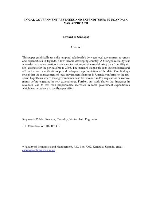
LOCAL GOVERNMENT REVENUES AND EXPENDITURES IN UGANDA: A<strong>VAR</strong> APPROACHEdward B. Sennoga†AbstractThis paper empirically tests the temporal relationship between local <strong>government</strong> <strong>revenues</strong><strong>and</strong> <strong>expenditures</strong> <strong>in</strong> Ug<strong>and</strong>a, a low <strong>in</strong>come develop<strong>in</strong>g country. A Granger-causality testis conducted <strong>and</strong> estimation is via a vector autoregressive model us<strong>in</strong>g data from fifty six(56) districts for the period 2001 to 2003. The st<strong>and</strong>ard diagnostic tests are conducted <strong>and</strong>affirm that our specifications provide adequate representation of the data. Our f<strong>in</strong>d<strong>in</strong>gsreveal that the management of local <strong>government</strong> f<strong>in</strong>ances <strong>in</strong> Ug<strong>and</strong>a conforms to the taxspendhypothesis where local <strong>government</strong>s raise tax revenue <strong>and</strong>/or request for or receivegrants before engag<strong>in</strong>g <strong>in</strong> new <strong>expenditures</strong>. Further, our study shows that <strong>in</strong>creases <strong>in</strong><strong>revenues</strong> lead to less than proportionate <strong>in</strong>creases <strong>in</strong> local <strong>government</strong> <strong>expenditures</strong>which lends credence to the flypaper effect.Keywords: Public F<strong>in</strong>ances, Causality, Vector Auto RegressionJEL Classification: H6, H7, C3† Faculty of Economics <strong>and</strong> Management, P.O. Box 7062, Kampala, Ug<strong>and</strong>a, email:esennoga@fema.mak.ac.ug
I. IntroductionFiscal policy is widely considered an <strong>in</strong>strument that can be used to alleviate short-termfluctuations of output <strong>and</strong> employment <strong>and</strong> br<strong>in</strong>g the economy closer to full employment(Zagler <strong>and</strong> Durnecker (2003)). This adjustment could proceed via changes <strong>in</strong> <strong>revenues</strong>,<strong>expenditures</strong> or both. On the revenue side, non-lump sum taxes can distort the behaviorof economic agents as regards the accumulation <strong>and</strong> supply of factors of production.However, distortionary taxation can <strong>in</strong>ternalize the effect of the externality on privatedecision rules, consequently <strong>in</strong>duc<strong>in</strong>g the efficient allocation of resources (Turnovsky(1996)). On the expenditure side, endogenous growth models considered some publicexpenditure categories to critical drivers of economic growth. Examples here <strong>in</strong>clude<strong>expenditures</strong> on public <strong>in</strong>frastructure, research <strong>and</strong> development, education <strong>and</strong> health(Barro (1990); Romer (1990); <strong>and</strong> Bloom et al. (2001)).When public <strong>expenditures</strong> exceed public <strong>revenues</strong>, the result<strong>in</strong>g deficit can be <strong>in</strong>terpretedas a means of f<strong>in</strong>anc<strong>in</strong>g additional <strong>government</strong> <strong>expenditures</strong>. If such <strong>expenditures</strong> areconsidered growth enhanc<strong>in</strong>g, then a <strong>government</strong> deficit exhibits an <strong>in</strong>direct effect onlong-term economic growth (Carneiro et al. (2005). However, <strong>in</strong> a Ricardian world whereagents view deficits only as taxes delayed, tax <strong>and</strong> deficit f<strong>in</strong>ance of <strong>government</strong> f<strong>in</strong>anceshould be identical especially if the tax structure rema<strong>in</strong>s unchanged <strong>in</strong> the future(Ludvigson (1996)). In a non-Ricardian economy, say, due to credit constra<strong>in</strong>ts oroverlapp<strong>in</strong>g generations, public debts can alter private <strong>in</strong>centives to accumulate factors ofproduction <strong>and</strong> thus directly <strong>in</strong>fluence the rate of growth of the economy. it is importantto note that a debt f<strong>in</strong>anced deficit could <strong>in</strong>duce the <strong>government</strong> to absorb additionalresources from the private sector, which could have been utilized <strong>in</strong>stead for theaccumulation of private capital (Araujo <strong>and</strong> Mart<strong>in</strong>s (1999)). However, the overallgrowth effect would be negative if the revenue raised <strong>in</strong> such a fashion is spent <strong>in</strong> a lessproductive way than it would have been by the private sector.This paper focuses on the <strong>in</strong>tertemporal relationship between <strong>revenues</strong> <strong>and</strong> <strong>expenditures</strong>.Four different hypotheses can be considered to exam<strong>in</strong>e such a problem. The “tax-spend”hypothesis postulates that <strong>government</strong>s raise tax <strong>revenues</strong> before to undertak<strong>in</strong>g new<strong>expenditures</strong> (Friedman (1978)); Buchanan <strong>and</strong> Wagner (1978)). The “spend-tax”hypothesis on the other h<strong>and</strong> suggests that <strong>government</strong>s engage <strong>in</strong> <strong>expenditures</strong> first <strong>and</strong>then <strong>in</strong>crease tax <strong>revenues</strong> to f<strong>in</strong>ance these <strong>expenditures</strong>. (Carneiro et al. (2005); Peacock<strong>and</strong> Wiseman (1979); <strong>and</strong> Barro (1974)). The “fiscal synchronization” hypothesispredicts that <strong>government</strong>s take decisions about <strong>revenues</strong> <strong>and</strong> <strong>expenditures</strong> simultaneously(Musgrave (1966); Meltzer <strong>and</strong> Richard (1981)). F<strong>in</strong>ally, fiscal <strong>in</strong>dependence regard<strong>in</strong>gthe decisions to spend <strong>and</strong> raise <strong>revenues</strong> is also a possible hypothesis (Baghestani <strong>and</strong>McNown (1994)).The nexus between <strong>government</strong> <strong>revenues</strong> <strong>and</strong> <strong>expenditures</strong> is an issue that has been<strong>in</strong>vestigated for several countries though a consensus is yet to be reached. Dhanasekaran(2001) <strong>and</strong> Carneiro et al. (2005) exam<strong>in</strong>ed the cases of India <strong>and</strong> Gu<strong>in</strong>ea Bissau,respectively. They report evidence <strong>in</strong> support of the spend-tax hypothesis. Ew<strong>in</strong>g <strong>and</strong>1
Payne (1998) have exam<strong>in</strong>ed the case of five Lat<strong>in</strong> American countries f<strong>in</strong>d<strong>in</strong>g mixedresults for this set of countries. Park (1998) found evidence <strong>in</strong> support of the tax-spendhypothesis for the case of Korea. The <strong>in</strong>tertemporal relationship between <strong>revenues</strong> <strong>and</strong><strong>expenditures</strong> is evidently an issue that is yet to be settled empirically.In the sections that follow, we test these hypotheses us<strong>in</strong>g annual central <strong>government</strong><strong>revenues</strong> <strong>and</strong> expenditure data for the period 1982-2006 as well as data from fifty six (56)districts <strong>in</strong> Ug<strong>and</strong>a for the period 2001-2003. Thus, our study exam<strong>in</strong>es the revenueexpenditurerelationship both at the national <strong>and</strong> sub national <strong>government</strong> levels. To thebest of our knowledge, this study is the only one that exam<strong>in</strong>es the revenue-expenditurenexus us<strong>in</strong>g both national <strong>and</strong> sub national <strong>government</strong> data.Ug<strong>and</strong>a was one of the <strong>in</strong>itial beneficiaries of the heavily <strong>in</strong>debted poor country (HIPCs)<strong>in</strong>itiative <strong>and</strong> has also been hailed by the IMF <strong>and</strong> World Bank for her remarkable growthfollow<strong>in</strong>g the civil strife that had engulfed the country <strong>in</strong> the early 1980’s. Consequently,this study aims to exam<strong>in</strong>e whether fiscal discipl<strong>in</strong>e <strong>and</strong> sound public f<strong>in</strong>ancemanagement could have been important factors engender<strong>in</strong>g <strong>in</strong> efficient resourceallocation <strong>and</strong> economic growth. The rem<strong>in</strong>der of this paper is organized as follows.Section II presents the methodology, the third <strong>and</strong> fourth Sections report the empiricalresults, conclusions, <strong>and</strong> policy implications, respectively.II. Empirical MethodologyThis study employs the vector autoregressive (<strong>VAR</strong>) <strong>and</strong> the Granger causality analysisdeveloped by Sims (1980) <strong>and</strong> Granger (1980). We apply the <strong>VAR</strong> together with theGranger-Causality method to test for Granger causality between <strong>government</strong><strong>expenditures</strong> <strong>and</strong> <strong>government</strong> <strong>revenues</strong> <strong>in</strong> Ug<strong>and</strong>a. Our estimated <strong>VAR</strong> model consists oftwo endogenous variables: <strong>government</strong> <strong>expenditures</strong> <strong>and</strong> <strong>government</strong> <strong>revenues</strong>. The <strong>VAR</strong>model is preferred over the simultaneous equations approach because the latter is largelyviewed to be too restrictive <strong>and</strong> the selection of endogenous <strong>and</strong> exogenous variables isarbitrary <strong>and</strong> can be subject to researcher’s preferences. However, for the <strong>VAR</strong>technique, all variables <strong>in</strong> the model are endogenous <strong>and</strong> each variable can be expressedas a l<strong>in</strong>ear function of its own lagged values <strong>and</strong> the lagged values of all other variables<strong>in</strong> the system (Cheng <strong>and</strong> Lai (1997)). An additional advantage of the <strong>VAR</strong> is that it hasbeen used to test for causality between two or more variables.The <strong>in</strong>vestigative approach adopted by this study consists of four major steps. First theaugmented Dickey Fuller, Phillips Perron (1988), <strong>and</strong> the KPSS (see Kwiatowski et al.(1992)) tests for stationarity are performed, second; the optimal lag length is determ<strong>in</strong>edus<strong>in</strong>g the Schwarz BIC model selection criterion (Stock (1994)); third, the Granger-Causality tests (see Granger (1980)) are implemented to estimate the pair wise causalityfor each equation; <strong>and</strong> fourth, we estimate the <strong>VAR</strong> model to test the causal relationshipbetween <strong>government</strong> <strong>expenditures</strong> <strong>and</strong> <strong>revenues</strong>.2
III. Data <strong>and</strong> Empirical ResultsAnnual data for 56 local <strong>government</strong>s (districts) is used to exam<strong>in</strong>e the <strong>in</strong>terrelationshipsbetween <strong>government</strong> <strong>revenues</strong> <strong>and</strong> <strong>expenditures</strong>. These local <strong>government</strong> data are for theperiod 2001-2003 <strong>and</strong> are obta<strong>in</strong>ed from <strong>Local</strong> Government Returns published by theM<strong>in</strong>istry of F<strong>in</strong>ance, Plann<strong>in</strong>g <strong>and</strong> Economic Development. Prior to 2006, the majorsource of revenue for local <strong>government</strong>s <strong>in</strong> Ug<strong>and</strong>a was the graduated tax—apresumptive tax—levied on each adult Ug<strong>and</strong>a 1 . Other revenue sources for local<strong>government</strong>s <strong>in</strong> Ug<strong>and</strong>a <strong>in</strong>cluded property taxes, user fees <strong>and</strong> charges such as tourismtaxes (for <strong>in</strong>stance on recreational facilities such as beaches), taxes on the transportationof produce, urban authority permits, license fees <strong>and</strong> market dues.Due to unavailability of consistent <strong>and</strong> comparable local <strong>government</strong> data on<strong>expenditures</strong>, we use transfers from the central <strong>government</strong> to proxy for local <strong>government</strong><strong>expenditures</strong>. Such transfers <strong>in</strong>clude equalization transfers, funds for rural feeder roads,primary health care, agricultural extension (National Agricultural Advisory Services),UPE, <strong>and</strong> transfers to pay salaries. Though it is true that districts could use own generatedfunds to f<strong>in</strong>ance <strong>expenditures</strong> other than those covered under the local <strong>government</strong>transfers, we do not expect substantial deviations of the “actual” <strong>expenditures</strong> from local<strong>government</strong> transfers especially s<strong>in</strong>ce the majority of local <strong>government</strong>s <strong>in</strong> Ug<strong>and</strong>a relyon central <strong>government</strong> transfers to f<strong>in</strong>ance their programmes.An obvious advantage of us<strong>in</strong>g local <strong>government</strong> data is that they depict revenue <strong>and</strong>expenditure variations over time as well as across (districts) local <strong>government</strong>s. It isanticipated that the additional variation will improve the quality of the estimated revenueexpenditurerelationship.1. Tests for StationarityLiterature shows that us<strong>in</strong>g non-stationary data <strong>in</strong> causality tests could yield spuriouscausality results. As emphasized by Park (1998), we first perform unit root tests on ourvariables before proceed<strong>in</strong>g with the Granger-causality test so as to avoid the spuriousregression problem <strong>and</strong> to account for the appropriate dynamic specification. Stationarityof the variables was tested us<strong>in</strong>g the Augmented Dickey-Fuller (ADF) <strong>and</strong> the Phillips-Perron (PP) tests. However, these tests have been criticized for their limited ability todist<strong>in</strong>guish between series that are purely non-stationary processes <strong>and</strong> those with nearunit roots. Thus, we also run the KPSS (1992) test which has the null of stationarity. Asmentioned above, the optimal lag length of the tests is determ<strong>in</strong>ed us<strong>in</strong>g the Schwarz BICmodel selection criterion as recommended by Stock (1994).Table 1 shows that the ADF <strong>and</strong> PP tests allow for the rejection of the null hypothesis ofnon-stationarity for the levels of the variables while <strong>in</strong> the KPSS test we do not reject thenull hypothesis of stationarity for the levels of the variables. Consequently, we conclude1 Exceptions here <strong>in</strong>cluded the housewives, those serv<strong>in</strong>g <strong>in</strong> the armed forces <strong>and</strong> those under <strong>in</strong>carceration.3
that our variables are stationary or <strong>in</strong>tegrated of order zero <strong>and</strong> we can then proceed withthe simplest version of the Granger-causality test us<strong>in</strong>g the levels of the variables.Table 1. Unit Root Tests for Levels of the Variables 2001-2003Variables ADF Phillips-Perron KPSS LagLengthLog levels: 1ln G -6.268 -6.341 0.107 1ln T -6.323 -6.354 0.0612 1Notes: The lag length was determ<strong>in</strong>ed by select<strong>in</strong>g the lowest Bayesian Information Criterion for each ofthe variables. The critical values for the different tests are: ADF <strong>and</strong> Phillips Perron 1% (-3.488); 5% (-2.886) <strong>and</strong> KPSS 1% (0.216); 5% (0.146).2. The Granger-Causality TestA test of causality is whether the lags of one variable enter <strong>in</strong>to the equation for anothervariable (Enders, 1995). Consider two series { k t} <strong>and</strong>{ l t}. If better predictions of { k t}k the current <strong>and</strong> lagged values ofcan be obta<strong>in</strong>ed by add<strong>in</strong>g to lagged values of { t}another variable { l }, then {} l is said to Granger cause { }ttk t. Stated differently, { t}said to precede temporally { kt} <strong>in</strong> that changes <strong>in</strong> { t}l t}{} l tdoes not improve the forecast<strong>in</strong>g performance of{ k t}, then { t}cause{ }.k tl isk follow the changes <strong>in</strong>{ . Thus, ifl does not GrangerTable 3 presents results from the Granger-causality tests which were obta<strong>in</strong>ed with onelag for each variable. Annual data for the period 2001-2003 reveals that causality isunidirectional for Ug<strong>and</strong>a’s local <strong>government</strong>s: <strong>revenues</strong> (T) affect <strong>expenditures</strong> but thereverse is not true.Table 2. Granger Causality Tests for Expenditures <strong>and</strong> Revenues: 2001-2003Hypothesis Test Statistic ConclusionExpenditures Granger-Cause Revenues t-prob = 0.092 RejectRevenues Granger-Cause Expenditures t-prob = 0.719 Do not reject3. The Vector Autoregression ModelThe <strong>VAR</strong> approach is adopted because the purpose of this study is to determ<strong>in</strong>e the<strong>in</strong>terrelationship among <strong>government</strong> <strong>expenditures</strong> (G) <strong>and</strong> <strong>revenues</strong> (T). Stateddifferently, we treat each variable (<strong>expenditures</strong> <strong>and</strong> <strong>revenues</strong>) symmetrically because weare not certa<strong>in</strong> which one is exogenous. As mentioned above, there is some evidence <strong>in</strong>support of both the “tax-spend” <strong>and</strong> “spend-tax” hypotheses. 2 We let the time path of2 For <strong>in</strong>stance see Buchanan <strong>and</strong> Wagner (1977), Friedman (1978), <strong>and</strong> Park (1998).4
{ G t} be affected by the current <strong>and</strong> past realizations of the { t}T sequence <strong>and</strong> the let thetime path of the { T t} sequence be affected by current <strong>and</strong> past realizations of the{ G t} sequence. Our simple bivariate system can be represented as a first order <strong>VAR</strong>3 asfollows:[1]G = bt10+ b12Tt+ γ G11t−1+ γ T12t−1+ εGt[2]T = bt20+ b21Gt+ γ G21t−1+ γ T22t−1+ εTtWhere (as verifed above), both G <strong>and</strong> are stationary <strong>and</strong> thetT { ε } <strong>and</strong> { ε }tuncorrelated white noise disturbances. Here, is the contemporaneous effect of a unitchange of T on <strong>and</strong> γ the effect of a unit change <strong>in</strong> G on T . In other words, thetGt21structure of this system <strong>in</strong>corporates feedback s<strong>in</strong>ce Gt<strong>and</strong> Ttare allowed to affect eachother. After some manipulation, the above structural <strong>VAR</strong> (equations [1] <strong>and</strong> [2]) can bereduced to follow<strong>in</strong>g st<strong>and</strong>ard form:b 12t−1tGtTtare[3]G = at10+ a11Gt−1+ a12Tt−1+ e1t[4]T = at20+ a21Gt−1+ a22Tt−1+ e2tS<strong>in</strong>ce equations [3] <strong>and</strong> [4] each have identical right-h<strong>and</strong>-side variables, estimation viaord<strong>in</strong>ary least squares technique will yield efficient estimates. Table 3 shows results fromthe <strong>VAR</strong> estimation <strong>and</strong> were obta<strong>in</strong>ed with one lag for each variable. The results <strong>in</strong>Table 3 confirm the uni-directional causation between <strong>expenditures</strong> <strong>and</strong> <strong>revenues</strong> withcausation runn<strong>in</strong>g from <strong>government</strong> <strong>revenues</strong> to <strong>government</strong> <strong>expenditures</strong>. In otherwords, local <strong>government</strong> <strong>revenues</strong> <strong>and</strong> <strong>expenditures</strong> are related by a feedback causalmechanism, <strong>and</strong> this is consistent with the tax-spend hypothesis <strong>in</strong>dicat<strong>in</strong>g that the local<strong>government</strong>s <strong>in</strong> Ug<strong>and</strong>a raise <strong>revenues</strong> first <strong>and</strong> then identify spend<strong>in</strong>g priorities.Table 3. <strong>VAR</strong> estimation results: 2001-2003Equationln <strong>revenues</strong> ln <strong>expenditures</strong>ln <strong>revenues</strong> 0.636(6.77)***0.067(1.68)*ln <strong>expenditures</strong> -0.077(0.36)0.505(5.54)***Constant 9.292 9.7272Adj. R 0.37 0.40Durb<strong>in</strong>-Watson 1.83 1.943 The optimal lag length was determ<strong>in</strong>ed us<strong>in</strong>g the Schwarz BIC model selection criterion.5
Prob (F-stat.) 0.0 0.0Number of observations 167 167Notes: Absolute value of z statistics <strong>in</strong> parentheses;* Significant at 10%; ** significant at 5%; *** significant at 1%.Further, the results reveal a low “tax-spend” elasticity. In particular, a 10 percent <strong>in</strong>crease<strong>in</strong> <strong>revenues</strong> results <strong>in</strong> a 1 percent <strong>in</strong>crement <strong>in</strong> <strong>expenditures</strong>. Though not the focus of thisstudy the <strong>in</strong>elastic response of <strong>expenditures</strong> to changes <strong>in</strong> <strong>revenues</strong> is has importantpublic f<strong>in</strong>ance implications. Public f<strong>in</strong>ance economists have come to refer to thisphenomenon by different names rang<strong>in</strong>g from the “fly paper” effect to mere abuse ofoffice <strong>and</strong>/ or corruption. The former school of thought is premised on the argument that“money tends to stick” where is l<strong>and</strong>s s<strong>in</strong>ce only a fraction of a given dollar of publicfunds utilized <strong>in</strong> the provision of public goods <strong>and</strong> services. Proponents of the latterschool of thought argue that the corruption <strong>and</strong> graft that has often plagued the publicsector is one s<strong>in</strong>gle most important reason for the absence of a one to one relationshipbetween <strong>revenues</strong> raised <strong>and</strong> public <strong>expenditures</strong>.4. Test<strong>in</strong>g for Autocorrelation <strong>in</strong> the ResidualsWe conduct a serial autocorrelation test <strong>in</strong> the residuals via the lagrange-mulitplier testwhich has a null hypothesis of no autocorrelation. The lagrange-multiplier test does notreject the null hypothesis of no autocorrelation <strong>in</strong> the residuals at the optimal lag order(one) which is consistent with a well specified model. The Chi-square statistic <strong>and</strong> p-values obta<strong>in</strong>ed at lag one (1) are 5.27 <strong>and</strong> 0.26, respectively, which does not allow forthe rejection the null hypothesis of no autocorrelation.Follow<strong>in</strong>g Engle <strong>and</strong> Granger (1987), we regress the first difference of the residuals onthe previous period disturbances. The test for unit root <strong>in</strong> the disturbances comprisestest<strong>in</strong>g whether the coefficient on the lagged disturbances is not statistically differentfrom zero. Failure to reject the null hypothesis that this coefficient is not statisticallydifferent from zero <strong>in</strong>dicates that the sequence of disturbance terms conta<strong>in</strong>s a unit root.Apply<strong>in</strong>g this procedure to our data leads to the rejection of the null hypothesis <strong>in</strong>dicat<strong>in</strong>gthat the residuals are stationary which rules out the null hypothesis of spuriousregression. 45. Discussion of the Empirical ResultsThe Granger-causality test <strong>and</strong> the <strong>VAR</strong> reveal unilateral causation between <strong>government</strong><strong>revenues</strong> <strong>and</strong> <strong>expenditures</strong> with causation runn<strong>in</strong>g from <strong>revenues</strong> to <strong>expenditures</strong> forUg<strong>and</strong>a’s local <strong>government</strong>s. In light of these f<strong>in</strong>d<strong>in</strong>gs, we can conclude that local<strong>government</strong>s <strong>in</strong> Ug<strong>and</strong>a follow the “tax-spend” hypothesis. The “tax-spend” hypothesismeans that local <strong>government</strong>s <strong>in</strong> Ug<strong>and</strong>a seem to raise tax revenue <strong>and</strong>/or request for orreceive grants before engag<strong>in</strong>g <strong>in</strong> new <strong>expenditures</strong>. The “tax-spend” hypothesis is <strong>in</strong> l<strong>in</strong>ewith the concept of budget framework papers which requires local <strong>government</strong>s to4 We reject the null hypothesis of unit root <strong>in</strong> the disturbances at the 1 percent level of significance.6
identify their spend<strong>in</strong>g priorities first, say, through <strong>Local</strong> Government budget frameworkpapers <strong>and</strong> budget conferences <strong>and</strong> then submit these requests to the Central Governmentfor fund<strong>in</strong>g or raise the requisite fund<strong>in</strong>g necessary to f<strong>in</strong>ance these expenditurepriorities.The “tax-spend” hypothesis implicitly pre-supposes that local <strong>government</strong>s <strong>in</strong> Ug<strong>and</strong>a donot run budget deficits s<strong>in</strong>ce their <strong>expenditures</strong> are aligned to available fund<strong>in</strong>g. This isespecially true <strong>in</strong> Ug<strong>and</strong>a s<strong>in</strong>ce local <strong>government</strong>s have limited access to both public(say, via the issuance of local <strong>government</strong> bonds) <strong>and</strong> private borrow<strong>in</strong>g. Consequently,local <strong>government</strong>s have to prioritize the use of any available f<strong>in</strong>ancial resources whichimproves fiscal discipl<strong>in</strong>e <strong>and</strong> controls the size of the local <strong>government</strong>s’ public deficits.However, <strong>in</strong> the absence of substantial transfers from the <strong>government</strong>, the limited abilityto raise revenue coupled with <strong>in</strong>adequate own revenue sources suggests that severalessential local <strong>government</strong> service delivery <strong>in</strong>itiatives will more than likely be suspended.Our f<strong>in</strong>d<strong>in</strong>gs are consistent with Park (1998) who found evidence <strong>in</strong> support of the taxspendhypothesis for the case of Korea. Our f<strong>in</strong>d<strong>in</strong>gs also reaffirm earlier studies byBuchanan <strong>and</strong> Wagner (1977) <strong>and</strong> Friedman (1978) who argue that <strong>government</strong>s firstraise tax <strong>revenues</strong> before engag<strong>in</strong>g <strong>in</strong> new <strong>expenditures</strong>.6. Conclusions <strong>and</strong> policy recommendationsIn this paper we assess the <strong>in</strong>tertemporal relationship between <strong>government</strong> <strong>expenditures</strong><strong>and</strong> <strong>revenues</strong> for Ug<strong>and</strong>a’s local <strong>government</strong>s. Quantify<strong>in</strong>g this relationship is important<strong>in</strong> as far as underst<strong>and</strong><strong>in</strong>g the role of <strong>government</strong> <strong>in</strong> allocation of resources is concerned.The fundamental premise of this paper is that the “sourc<strong>in</strong>g” of local <strong>government</strong><strong>revenues</strong> precedes the spend<strong>in</strong>g of these <strong>revenues</strong> by local <strong>government</strong> <strong>expenditures</strong> <strong>in</strong>Ug<strong>and</strong>a, which is also known as the tax-spend hypothesis.This objective is achieved <strong>in</strong> several steps. First, us<strong>in</strong>g data for the period 2001-2003from fifty six (56) local <strong>government</strong>s <strong>in</strong> Ug<strong>and</strong>a, we are unable to reject the tax-spendhypothesis. Second, our econometric tests further reveal that while there is a stable longrunrelationship between local <strong>government</strong> <strong>revenues</strong> <strong>and</strong> <strong>expenditures</strong>, there existsunilateral casualty runn<strong>in</strong>g from <strong>government</strong> <strong>revenues</strong> to <strong>expenditures</strong>. Stated differently,local <strong>government</strong>s <strong>in</strong> Ug<strong>and</strong>a face limited risk of budget deficit explosions over the longterm<strong>and</strong> this could be due to the fact that these sub-national <strong>government</strong>s raise funds first<strong>and</strong> subsequently f<strong>in</strong>ance <strong>expenditures</strong>.Our results po<strong>in</strong>t to the importance of align<strong>in</strong>g both local <strong>and</strong> central <strong>government</strong><strong>expenditures</strong> with revenue mobilization capacity. Such alignment will also to improveefficiency <strong>in</strong> the allocation of resources particularly to the growth-enhanc<strong>in</strong>g categories<strong>in</strong>clud<strong>in</strong>g <strong>in</strong>frastructure, health <strong>and</strong> education. The result<strong>in</strong>g control over <strong>expenditures</strong>rather than an <strong>in</strong>crease <strong>in</strong> tax <strong>revenues</strong> will enhance Ug<strong>and</strong>a’s fiscal discipl<strong>in</strong>econsequently foster<strong>in</strong>g an effective medium term budget<strong>in</strong>g framework.7
ReferencesAraujo, J. T., <strong>and</strong> M.A.C. Mart<strong>in</strong>s (1999), Economic Growth with F<strong>in</strong>ite Lifetimes,”Economic Letters, 62, 377-381.Baghestani, H., <strong>and</strong> R. McNown (1994), “Do Revenues or Expenditures Respond toBudgetary Disequilibria?” Southern Economic Journal, 311-322.Barnhart, S. W., <strong>and</strong> A. F. Darrat (1989), “Federal Deficits <strong>and</strong> Money Growth <strong>in</strong> theUnited States,” Journal of Bank<strong>in</strong>g <strong>and</strong> F<strong>in</strong>ance, 13, 311-322Barro, R. J. (1974), “Are Government Bonds Net Wealth?” Journal of PoliticalEconomy, 82, 1095-1118.__________(1990), “Government Spend<strong>in</strong>g <strong>in</strong> a Simple Model of Endogenous Growth,”Journal of Political Economy, 98.Bloom, D. E., D. Cann<strong>in</strong>g, <strong>and</strong> J. Sevilla (2001), “The Effect of Health on EconomicGrowth: Theory <strong>and</strong> Evidence,” National Bureau of Economic Research,Work<strong>in</strong>g Paper No. 8587.Buchanan, J., <strong>and</strong> R. Wagner (1977), Democracy <strong>in</strong> Deficit, New York: Academic Press.Carneiro, F. G., J.R. Faria, <strong>and</strong> B.S. Barry (2005), “Government Revenues <strong>and</strong>Expenditures <strong>in</strong> Gu<strong>in</strong>ea-Bissau: Causality <strong>and</strong> Co<strong>in</strong>tegration,” Journal ofEconomic Development, 30(1), 107-117.Cheng, B. S., <strong>and</strong> T. W. Lai (1997), “Government Expenditures <strong>and</strong> Economic Growth <strong>in</strong>South Korea: A <strong>VAR</strong> Approach,” Journal of Economic Development, 22(1), 11-24.Dhanasekaran, K. (2001), “Government Tax Revenue, Expenditure <strong>and</strong> Causality: TheExperience of India,” India Economic Review, 2, 359-379.Enders, W, (1995), Applied Econometric Time Series, John Wiley & Son, Inc.Engle, R. F., <strong>and</strong> C. W. J. Granger (1987), “Co<strong>in</strong>tegration <strong>and</strong> Error-Correction:Representation, Estimation <strong>and</strong> Test<strong>in</strong>g,” Econometrics, 55, 251-276.Ew<strong>in</strong>g, B., <strong>and</strong> J. Payne (1998), “Government Tax Revenue-Expenditure Nexus:Evidence from Lat<strong>in</strong> America,” Journal of Economic Development, 23, 57-69.Friedman, M. (1978), “The Limitations of Tax Limitation,” Policy Review, 7-14.8
Granger, C. W. (1980), “Test<strong>in</strong>g for Causality,” Journal of Economic Dynamics <strong>and</strong>Control, 4, 229-252.Kwiatkowski, D., P.C.B. Phillips P. Schmidt, <strong>and</strong> Y. Sh<strong>in</strong> (1992), Test<strong>in</strong>g the nullhypothesis of stationarity aga<strong>in</strong>st the alternative of a unit root: How sure are wethat economic time series have a unit root?” Journal of Econometrics, 54: 159-178.Ludvigson, S. (1996), “The Macroeconomic Effects of Government Debt <strong>in</strong> a StochasticGrowth Model,” Journal of Monetary Economics, 38, 25-45.Lutkepohl, H. (1982), “Non-Causality Due to Omitted Variables,” Journal ofEconometrics, 19, 367-378.Musgrave, R. (1996), “Pr<strong>in</strong>icples of Budget Determ<strong>in</strong>ation,” <strong>in</strong> H. Cameron <strong>and</strong> W.Henderson, Public F<strong>in</strong>ance: Selected Read<strong>in</strong>gs, New York: R<strong>and</strong>om House.Meltzer, A., <strong>and</strong> S. Richard (1981), “A Rational Theory of the Size of the Government,”Journal of Political Economy, 89, 914-927.Park, W. (1998), “Granger Causality between Government Revenues <strong>and</strong> Expenditures <strong>in</strong>Korea,” Journal of Economic Development, 23, 145-155.Peacock, A., <strong>and</strong> J. Wiseman (1979), “Approaches to the Analysis of GovernmentExpenditures Growth,” Public F<strong>in</strong>ance Quarterly, 3-23.Romer, P.M. (1990), “Endogenous Technological Change,” Journal of PoliticalEconomy, 98, 71-102Sims, C. A. (1980), “Macroeconomics <strong>and</strong> Reality,” Econometrica, 48, 1-48.Stock, J. (1994), “Unit roots, structural breaks <strong>and</strong> trends,” <strong>in</strong> Engle, R. <strong>and</strong> McFedden,D. (eds.) H<strong>and</strong>book of Econometrics, Volume 4: 2739-2841, Elsevier,Amsterdam.Turnovsky, S.J. (1996), “The Effect of Taxation on Human Capital,” Journal of PublicEconomics, 60, 21-44Zagler, M., <strong>and</strong> Durnecker (2003), “Fiscal Policy <strong>and</strong> Economic Growth,” Journal ofEconomic Surveys, 17, 397-422.9


