Fiscal policy rules for managing oil revenues in Nigeria

Fiscal Policy Rules for Managing Oil
Revenues in Nigeria
Moses Obinyeluaku 1
University of Cape Town
Nicola Viegi 2
University of Cape Town and ERSA
Abstract
Nigeria is heavily dependent on oil revenue to finance over 80 per cent of its
total expenditure, making its budget vulnerable to fiscal shocks. This poses a
serious threat both to the sustainability of the country’s budget and to its
macroeconomic stability. Oil windfall induces government spending that is
difficult to retrench when the oil revenue falls, distorting government budget
allocation pattern, cohesion and stability and increase deficits and debt stock
that has often created an unfavorable environment for monetary policy. The
question then is what form of fiscal policy rules will perform better in reducing
debt accumulation and promote the necessary medium-term budget deficit
stability. Theoretically, Basci et al (2004) proposed two alternative fiscal policy
rules in terms of their impact on debt sustainability: a rule that fixes the ratio of
primary surplus to GDP (“fixed surplus rule”) and one that sets the primary
surplus as a linear function of debt to GDP ratio (“variable surplus rule”). In
this paper, we extend the analysis looking at the effect of being dependent on
natural resource revenues on the sustainability of the two rules. A simple debt
dynamic equation, incorporating real shocks and oil price dynamic, is
constructed, and the probability of exceeding the steady state debt level is
simulated using Monte Carlo technique. The results show that the fixed surplus
rule performs better than the simple variable surplus rule when real interest rate
is relatively high and the ability to adjust government expenditure is limited.
Keywords: Fiscal Policy Rules, Debt sustainability, Monte Carlo Simulation,
Nigeria
JEL Classification: E61, E62, H62, H63.
1 mogalink@yahoo.com : I wish to acknowledge financial support by Codesria during the
preparation of this paper
2 nicola.viegi@uct.ac.za
1

1. INTRODUCTION
Macroeconomic dynamic in Nigeria has been dominated in the past by fiscal
instability. There have been a strong deficit and debt bias stemming from
government revenue volatility. As a result, monetary authority has been forced
to implement neutralizing monetary policies leading to macroeconomic
instability. 3
Policies adopted in response to high debt levels among the emerging and
developed countries vary. Brazil and Turkey have used the fixed primary
surplus rule, which fixes the ratio of primary budget surplus to GDP (Basci et
al, 2004). Argentina and Peru have applied limits to the overall balance and
primary expenditure. New Zealand has rules for the operating balance as well
as debt limits. 4 There is also the Stability and Growth Pact in the European
Union, though the issue of flexibility is beginning to appear in the practical
application of the constraints. 5
Drawing on this literature, the paper illustrates the appropriate fiscal policy
rules that will perform better in reducing debt accumulation and promote the
necessary medium-term budget deficit stability in Nigeria. It intends to
supplement a similar work by Baunsgaard (2003). 6
The paper compares the performance of the fixed primary surplus rule to an
alternative, the variable primary surplus rule, under which the primary budget
surplus is explicitly defined as an increasing function of the debt-to-GDP ratio,
using Monte Carlo technique. However, since government revenue in Nigeria
is exogenously given, the paper deviates a bit from the existing literature by
decomposing the primary surpluses into gross budgetary revenue and non-
3 See Batini (2004) and Obinyeluaku (2006)
4 See Kopits and Symansky (1998) and Kopits (2001).
5 See Dixit and Lambertini (2003) for more details.
6 He designed a fiscal rule nested within the long-run sustainable use of oil revenue in Nigeria.
2

interest budgetary expenditure in order to capture not only the volatility in
revenue via oil price dynamic, but also to control for the government
expenditure. 7 At least, for any fixed (variable) primary surplus rule, there is also
the level of fixed (variable) budgetary expenditure necessary to maintain such
rule. Shocks to real economy and oil prices are incorporated in the model. 8 As
the criterion of comparison, we use the probability of exceeding the sustainable
debt level at the end of the simulation horizon starting from a given initial debt
level.
The results show that in general the variable surplus rule performs better than
the simple fixed surplus rule, by reducing debt accumulation and the necessary
medium-term primary surplus. On the other hand a fix surplus rule works better
when the real interest rate is relatively high, i.e. when the explosive behavior of
debt dynamic is especially pronounced: With both rules fiscal stability implies a
marked increase in expenditure variability, more pronounce for the variable
interest rule. This result suggests that the government’s ability to make a
credible commitment to a fiscal rule depends on the flexibility of fiscal
expenditure.
The paper is organized as follows. Section II provides a brief overview of past
fiscal policy in Nigeria. Section III develops the model, and the analytical
definitions of the two fiscal rules and debt sustainability. The results of the
numerical simulations are presented in section IV and V. Section VI concludes.
II THE FISCAL STANCE
The past two decades have witnessed a considerable increase in government
indebtedness in Nigeria. Beyond the issue of poor quality of public
7 Fiscal policy rules could play a role in stabilizing expenditure programs at level consistent
with the necessary medium-term deficit stability.
8 A fiscal rule targeting a certain overall or primary fiscal balance in Nigeria without taking into
account, oil revenue volatility, will not prevent procyclical fiscal policies (Baunsgaard, 2003).
3

expenditure, the ability to save windfalls from excess crude oil proceeds by the
government remains critical in ensuring that government expenditure is
maintained at a sustainable level and consistent with the absorptive capacity of
the economy.
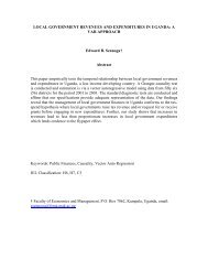
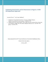
Figure 1a reveals that there is a substantial increase in government spending,
primary deficit and debt in Nigeria between 1980 and 2005. The oil windfall
between 1990 and 1992 was followed by rapid growth in government spending
with an average of about 21 percent of GDP during that period. However, as the
oil market weakened in the subsequent years, oil receipts were not adequate to
meet increasing levels of demands, and expenditures being reinforced by
political pressures, were not rationalised. Government resorted to borrowing
mainly from the central bank to finance the huge deficits (see figure 1b).
From figure 1b, the CBN absorbs almost half of the Nigerian public debt
following Commercial bank and the public. This implies that government is
mainly financing its huge deficits through seigniorage − the so called “fiscal
indiscipline.” And when government prints money (or use seigniorage), it
increases the money supply and this in turn causes inflation.
Although the democratically elected government in 1999 adopted policies to
restore fiscal discipline, the rapid monetization of foreign exchange earnings
between 2000 and 2004, another era of oil windfall, resulted in a large increases
in government spending. In 2005 alone, government spending increases to 19
percent of GDP from 14 percent in 2000. Extra budgetary outlays not initially
included in the budget increased. Worst till, most of this spending are not
directed towards capital and socio-economic sectors.
Corollary, primary deficit worsened from an average of 2.6 percent of GDP in
1980s to one of 6.2 percent in 1990s. In 2002 alone, primary deficit increases
to 5 percent of GDP from 2 percent in 2000. This increase in deficits results in
4

a mounting stock of debt, ranging from 88 percent of GDP in 1980s to 96
percent of GDP in 1990s. In 2002 alone, the shock of debt increases to 91 per
cent of GDP from 45 per cent in 2000. However, considering the uncertain
fiscal dynamics in Nigeria, the recent fiscal adjustment witnessed in 2005 might
still not be sustained.
Nigeria’s fiscal revenues are largely coincided with oil revenue accounting for
nearly 80 percent of government revenues, which implies that the economy is
highly exposed to price fluctuations in the world oil markets. Naturally, oil
revenue is very volatile due to world oscillation in oil prices and to
unpredictable changes in OPEC assigned oil quota − of which Nigeria has been
a member since 1958 following the commercial discovery of oil in Ofoibiri in
River State, Nigeria in 1956.
Absent suitable fiscal rules and a proper finance-management framework for oil
related risks over the past two decade in Nigeria have led to boom-and-busttype
fiscal policies that have generated large and unpredictable movements in
government finances. 9 Consequently, this has been a recurrent source of
destabilizing effect of fiscal surprises on the domestic prices and exchange rate
as well as financial system. 10
9 Also see Katz (2003)
10 See Welcome Address by the former CBN Governor, Dr. J. Sanusi on 2004 Federal
Government Budget, and an Address by the New CBN Governor, Prof. C.C. Soludo, on the
Bankers’ Committee Meeting, July 2004).
5

Figure 1
(a) Nigeria Fiscal Trends, 1980-2005 (% of GDP)
(b) Holdings of the Nigeria’s Governments Domestic Debt by the Central
Bank, Commercial Bank and Public (Percentage of GDP
30.0
25.0
20.0
15.0
10.0
5.0
0.0
-5.0
1980
1981
1982
1983
1984
1985
1986
1987
1988
1989
1990
1991
1992
1993
1994
1995
1996
1997
1998
1999
2000
2001
2002
2003
2004
2005
cbn comercial public
6

III FISCAL RULES WITH UNCERTAIN REVENUES
There is an abundant academic literature on why unconstrained discretion over
fiscal policy can erode public finances and create unfavourable environment for
monetary policy and macroeconomic stability. The bottom line is that there is
generally a strong pressure on expanding government expenditure, a reluctance
to raise taxes to the extent necessary to fully finance public undertakings (often
referred to as fiscal illusion and a deficit bias) and the possibility of an inflation
bias.
As monetary policy rule intend to limit the ability of monetary authority to act
discretionally, so fiscal policy rules will – if observed – mitigate the
government’s tendency to abandon previous policy commitment. They seek to
confer credibility on the conduct of macroeconomic policies by removing
discretionary interventions. Their goal is to achieve trust by guaranteeing that
fundamentals will remain predictable and robust regardless of the government
in power. Thus, fiscal policy rules are particularly helpful if the government is
not able to guarantee a prudent fiscal policy to the economic sectors. It thus
seems appropriate to study the sustainability of simple fiscal rules in a case like
Nigeria, where the first source of macroeconomic instability is certainly the
dynamic of fiscal policy.
A. FISCAL POLICY WITH STOCHASTIC REVENUES
The possible way to model fiscal policy in Nigeria is to consider the stochastic
nature of government revenues that we have illustrated in the previous section.
Since about 80 percent of government revenues come from oil, we can safely
assume that total gross budgetary revenues equal to
GR
t
⎛
Pt
Q − ⎞
t
=
⎜ ⎝ ⎠
⎟ . (1) 7

Where
Q −
is the quantity of oil,, assumed to be fixed,
t
11 and P t is its price.
Thus, primary surplus at the end of the budget year is equal to:
−
⎛ ⎞
PSt = Pt⎜Q t⎟−Gt ⎝ ⎠
(2)
The government in each year has to plan expenditure G t on the basis of a
forecast of oil revenues for the period. If we assume that the price of oil follow
a pure random walk,
P = P −1
+ v , as our unit root test results shows, this
t
t
implies that the best forecast of oil price is equal to so E t
( P t
) = P t −1
this, the expected primary surplus at the beginning of budget year is;
t
. Following
−
⎛ ⎞
=
⎜ t ⎟
)
⎝ ⎠
( PS t
) E t
⎜ P ⎟
−1
− E t
( G t
E t −1 Q −1
(3)
or,
−
⎛ ⎞
Et
−1( PSt
) = P ⎜
t 1 Q ⎟
−
− Et
1( Gt
),
t
−
(3b)
⎝ ⎠
The inability to control fiscal revenues introduce a significant element of
uncertainty in the budgetary process, equal to the volatility of oil prices v t . Any
fiscal rule, in this context, should be tested using the budgetary process
described by equation (3).
Once government expenditure decision and oil prices are determined, the
resulting primary surplus will give the following debt dynamic.
11 Being exogenous and determined by OPEC not the government.
8

= + 1 ( 1 + )( − ) t
D R D PS , (4)
t t t
where, R t is the real interest rate in period t and D t is the debt stock at the
beginning of the period t. Both PS t and D t are in real terms. To express (4) in
term of output ratio we assume a constant growth rate of output. The path of
real output is then given by
( t
) Y t
Y t + 1
= 1+ g , (5)
where g t is the constant growth rate. Defining, the debt to GDP ratio as d t = D t /
Y t and combining (4) and (5),
⎣( ) ( ) ⎦ ( ps t )
dt+ 1
= ⎡ 1+ rt 1+ gt ⎤ dt
−
, (6)
where ps t =PS t / Y t .
To facilitate the comparison of our results with the one in Basci et al (2004), we
maintain the assumption that R t and g t have random components. We therefore
can define the random variable r t
through the following decomposition:
+ ε , the growth adjusted real interest rate,
t
t
t
( 1+
Rt
)
( 1+
g )
1+
r + ε = , (7)
t
where r t is the deterministic component of the real growth adjusted interest rate,
and є t is a zero mean independently and identically distributed (iid) random
variable which represents the interest rate, and growth shocks.
9

Next, assume that the deterministic component of the growth adjusted mean
real interest rate r(d t ) is an increasing function of the debt to GDP ratio. 12
t
( d t
r = r ) with r ’ (d t )>0, (8)
where r ’ (d t ) represents the first derivative of r(d t )
Combining (6), (7) and (8), we obtain,
d
( 1+
r( d
t
) +
t
)( dt
− pst
)
1
=
, (9)
t+ ε
where d t denotes debt to GDP ratio at the beginning of period t, and ps t denotes
the ratio of primary surplus to GDP in period t. It is assume that growth
adjusted mean real interest rate, r(d t ) is an increasing function of the debt to
GDP ratio.
Since the analysis here is limited to a developing country, like Nigeria, a linear
function of debt stock is assumed, for simplicity. 13
r
( d t
) ρdt
= For all t, (10)
where 0 < ρ

and combining (9), (10) and (11) we obtain
2
c
ρ d − ρd
ps − ps ,
(12)
c
t
t
B. FISCAL POLICY RULES
As in the Basci et al (2004), two alternative policy rules are considered:
(1) Fixed Primary Surplus Rule
The fixed primary surplus rule is equal to a constant s percent of GDP at every
period: ps t = s for all t, and in our case is
ps
t
= s = P
⎛
⎝
⎞
⎠
−
t −1 ⎜Qt
⎟ − Gt
, (13)
Now by controlling for G t , 15 our fixed expenditure rule now becomes
G
t
−
⎡ ⎛ ⎞⎤
= ⎢Pt
−1 ⎜Qt
⎟⎥
− s , (14)
⎣ ⎝ ⎠⎦
and fixed primary surplus rule, revenue at time t (GR t ) minus fixed
expenditure rule (which is G t ). Equation (14) is the level of expenditure
necessary in order to maintain a fixed primary surplus rule. The Critical debt
level for the fixed primary surplus rule 16 is the value of debt that solve the
following quadratic equation;
2
c
ρ d − sρd
− s = 0 , (15)
c
15 We cannot control for P t (Q t ) due to oil price volatility.
16 Obtained by taking ps t = s into (12)
11

which can be calculated as,
⎛
2
ρ ( ρ ) 4 ρ ⎞
⎜ s + ⎜ ⎛ s + s ⎟⎞
⎟
⎝ ⎝
⎠
d =
⎠
c
, (16)
2ρ
2 +
as s, ρ > 0 so that sρ
( sρ
) 4sρ
< .
:
(2) Variable Primary Surplus Rule
A variable fiscal rule adjusts the expected level of fiscal surpluses to the
outstanding level of debt so that a higher fiscal surplus (a tighter fiscal policy)
is set as the debt stock increases: a simple linear expression of that could be
ps
= σ for all t, σ > 0.
t
d t
Substituting σd t for s in (14), then; our variable expenditure rule will look
like;
G
t
−
⎡ ⎛ ⎞⎤
= ⎢Pt
−1 ⎜Qt
⎟⎥
−σdt
, (17)
⎣ ⎝ ⎠⎦
and variable primary surplus rule, revenue at time t minus variable
expenditure rules. Again, (17) is the level of expenditure necessary in order to
maintain a variable primary surplus rule.
With this rule the Critical debt level 17 is:
'
c
( − σ )
d = σ ρ 1
(18)
17 Again, obtained by taking ps t = σd t into (12)
12

When d t > d c , debt level blows up, and it tends to decline when d t < d c under
both fiscal rules. 18
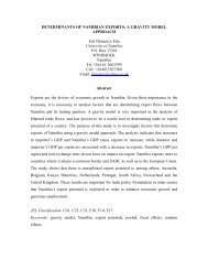
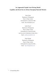
Note that which one of the two rules is more stringent depends critically on the
level of sensitivity of real interest rate to the level of debt ρ. As we can see from
the following numerical representation of the two functions (with parameters
values equal to the one used in the simulations that follows), for low level of ρ
(and consequently low level of real interest rate at any level of debt), a variable
fiscal rule offers a much less stringent constraint to the policy maker. The
opposite is true at the opposite end of ρ range, where is now the fix fiscal rule
that is a less stringent rule. This is somehow paradoxical: the variable rule, with
a built in adjustment mechanism, should by definition give more room of
manoeuvre to the policy maker. At the same time high interest rate penalizes
very significantly any increase in debt level so that the feedback mechanism in
the variable rule might not be fast enough to respond to a change in direction of
the debt dynamics. This is not quite intuitive and the simulations will help in
explaining this paradox.
18 As already proved in Basci et al (2004).
13

Figure 2 : Critical Level of Debt and Sensitivity of Real Interest Rate to Debt
Stock
IV SIMULATION RESULTS
The model illustrated in the previous sections is used to conduct simulations for
both fiscal rules using Monte Carlo techniques, for initial debt ratios (d 0 )
ranging from 20 percent of GDP to 100 percent of GDP. To perform the
simulations we calibrate initial oil price level so that the government revenues
at the beginning of the simulation amount to 20 percent of GDP, which is the
average government revenue in Nigeria for the past 10 years. The two shocks in
the model, oil shock v t and real rate shock є t , are assumed to be normally
distributed with zero mean and 2.5 percent variance and 5 percent respectively.
The debt ratio is than calculated using equation (9); and 1000 replications of a
14

five year horizon debt dynamic are computed. Arithmetic averages and standard
deviations of these trials are used in the quantitative analysis.
In other to capture the sensitivity of both rules to real interest rate levels, the
simulations are conducted with ρ at 10 percent and 15 percent, so that with a
baseline debt to GDP ratio of 60 percent, the growth adjusted real interest rate
is 6 percent (low) and 9 percent (high) respectevely.
For the numerical simulations, we set the parameters for both fiscal policy rules
as follows:
Fixed Rule:
⎡ ⎛
Gt Pt 1
Q − ⎞⎤
= ⎢ − ⎜ t⎟
⎝ ⎠
⎥− s , s = 0.04 corresponding to d c = 0.6528
⎣ ⎦
Variable Rule:
G
t
−
⎡ ⎛ ⎞⎤
= ⎢Pt
−1 ⎜Qt
⎟⎥
−σdt
, σ = 0.0667, corresponding to d ’ c = 0.7143
⎣ ⎝ ⎠⎦
The main result of the simulation is shown in table 1. Starting with a 60% level
of debt to gdp ratio and with ρ=0.1, the variable rule minimize substantially the
risk of debt exceeding the critical value. On the other hand the Variable rule
performs very badly once ρ is increased to 0.15. The probability of exceeding
the critical debt level at the next period (or medium-term) is less than 2 percent
for the variable rule, but more than 15 percent for the fixed, when the
simulation start from an initial debt ratio of 60 percent of GDP. 19 However,
although both rules explodes from an initial debt ratio of 60 percent of GDP at
higher real interest rate (that is r ≥ 9 percent), the probability of exceeding the
critical debt region is much higher with variable rule than fixed rule. Although
19 We compute our probabilities using the formulae,
Z
X − µ
σ
X
= , where X is the critical
debt level, µ is the average and σ is the standard deviation, from the simulation results.
X
15

the result shown is probably at the extreme end of the distribution, the observed
inversion of the ranking of the two rules is robust to any parametric
specification as can be seen in table 2 for the initial level of debt of 50%.
This result seems at odd with the intuition and with the similar contribution of
Basci et al (2004). The reason for this is that in our model the probability to be
affected by an adverse shock is reinforced by the presence of significant
uncertainty in the revenue collection. In this set up, a variable rule introduce an
extra element of variability in the debt dynamic that can be very penalising at
high level of real interest rate
Table 1: Probability Distribution outside the Critical Debt Value in the Medium-term
(Initial debt ratio 60%)
Fixed Rule
Variable Rule
ρ=0.1 13% 2%
ρ=0.15 86% 99%
Table 2: Probability Distribution outside the Critical Debt Value in the Medium-term
(Initial debt ratio 50%)
Fixed Rule
Variable Rule
ρ=0.1 0% 0%
ρ=0.15 19% 69%
16

30.00%
30.00%
25.00%
Critical debt
25.00%
20.00%
20.00%
Freq uency
15.00%
Freq uency
15.00%
10.00%
10.00%
5.00%
5.00%
Critical debt
0.00%
0.42 : 0.46 0.46 : 0.49 0.49 : 0.53 0.53 : 0.57 0.57 : 0.61 0.61 : 0.65 0.65 : 0.69 0.69 : 0.72 0.72 : 0.76 0.76 : 0.80
Debt - Fixed Rule
0.00%
0.44 : 0.47 0.47 : 0.51 0.51 : 0.55 0.55 : 0.58 0.58 : 0.62 0.62 : 0.66 0.66 : 0.70 0.70 : 0.73 0.73 : 0.77 0.77 : 0.81
Debt - Varialbe Rule
30.00%
25.00%
25.00%
20.00%
20.00%
15.00%
Frequency
15.00%
Critical debt
Frequency
10.00%
Critical debt
10.00%
5.00%
5.00%
0.00%
0.37 : 0.41 0.41 : 0.46 0.46 : 0.50 0.50 : 0.55 0.55 : 0.59 0.59 : 0.64 0.64 : 0.68 0.68 : 0.73 0.73 : 0.77 0.77 : 0.82
Debt - Fixed Rule
0.00%
0.41 : 0.44 0.44 : 0.47 0.47 : 0.51 0.51 : 0.54 0.54 : 0.58 0.58 : 0.61 0.61 : 0.64 0.64 : 0.68 0.68 : 0.71 0.71 : 0.74
Debt - Varialbe Rule
Figure 3: Probability Distribution of 60% Initial Debt Ratio at Next Period
and Medium Term with Low Real Interest Rate
17

30.00%
30.00%
25.00%
25.00%
20.00%
Critical debt
20.00%
Freq uency
15.00%
Freq uency
15.00%
10.00%
10.00%
Critical debt
5.00%
5.00%
0.00%
0.46 : 0.50 0.50 : 0.54 0.54 : 0.57 0.57 : 0.61 0.61 : 0.65 0.65 : 0.69 0.69 : 0.73 0.73 : 0.76 0.76 : 0.80 0.80 : 0.84
Debt - Fixed Rule
0.00%
0.45 : 0.49 0.49 : 0.53 0.53 : 0.56 0.56 : 0.60 0.60 : 0.64 0.64 : 0.68 0.68 : 0.72 0.72 : 0.76 0.76 : 0.80 0.80 : 0.84
Debt - Varialbe Rule
30.00%
30.00%
25.00%
25.00%
20.00%
Critical debt
20.00%
Frequency
15.00%
Frequency
15.00%
10.00%
10.00%
Critical debt
5.00%
5.00%
0.00%
0.43 : 0.48 0.48 : 0.54 0.54 : 0.59 0.59 : 0.64 0.64 : 0.70 0.70 : 0.75 0.75 : 0.80 0.80 : 0.86 0.86 : 0.91 0.91 : 0.96
0.00%
0.42 : 0.47 0.47 : 0.51 0.51 : 0.56 0.56 : 0.61 0.61 : 0.66 0.66 : 0.70 0.70 : 0.75 0.75 : 0.80 0.80 : 0.84 0.84 : 0.89
Debt - Fixed Rule
Debt - Varialbe Rule
Figure 4: Probability Distribution of 60% Initial Debt Ratio at Next Period
and Medium Term with High Real Interest Rate
18

V FISCAL RULES AND EXPENDITURE VARIABILITY
In our set up, where fiscal revenues are uncertain, the focus switches to fiscal
expenditure as the instrument in the hand of the government to satisfy any fiscal
constraint. The nature of the two rules analysed can be better understood if we
look at the volatility in expenditure plans that they require for the rule to be
satisfied. Table 3 and 4 illustrate the variability of expenditure for the two rules
in the case of low or high real interest rate and for all the different levels of
initial debt that we have simulated. In all cases, and naturally, the variability in
expenditure generated by the variable rule is higher than the one generated by
the fixed rule 20
Table 3: The Coefficient of Variation for both Rules in the Medium-term with Low
Real Interest Rate
Initial debt ratio Fixed expenditure rule Variable expenditure rule
20 0-164 0.181
30 0.169 0.179
40 0.176 0.183
50 0.170 0.179
60 0.168 0.179
Table 2: The Coefficient of Variation for both Rules in the Medium-term with High
real Interest Rate
Initial debt ratio Fixed expenditure rule Variable expenditure rule
20 0.174 0.185
30 0.175 0.192
40 0.168 0.182
50 0.164 0.175
60 0.169 0.190
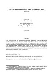
This implies that higher variability in government expenditure (between 15%
and 20%) is required in order to achieve and maintain the variable rule.
20 The coefficient of variation (CV) for both rules is measured by σ / µ, from the simulations.
19

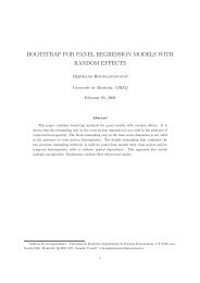
Indeed, figure 4 confirms that for the past two decades, the lowest level of debt
to GDP in Nigeria coincides with high variability in government expenditure. 21
1.8
1.6
1.4
1.2
1
0.8
0.6
0.4
0.2
0
80 81 82 83 84 85 86 87 88 89 90 91 92 93 94 95 96 97 98 99 2000 2001 2002 2003 2004
coeff var debt stock
Figure 4: Nigeria Debt and Coefficient of Variation on Government Expenditure (% of
GDP) 1980-2004
The stock of debt averaged from 63 percent of GDP between 1984 and 1985
(when CV on government expenditure is about 50 percent) to 118.3 and 124.2
between 1986-90 and 1990-94 (when CV ranges from 10 to 20 percent only).
Between 1995 and 1997, another period of high variability on government
expenditure (about 40 percent), the stock of debt averaged 55 percent of GDP.
In 1999 alone, when CV is about 45 percent, the stock of debt is only 32.5
percent compared with 73.2 percent in 2004 with less than 10 percent
variability.
21 This time, measured by the same formulae but based on the Nigeria data, 1980-2004 and not
on the simulation results..
20

VI CONCLUSIONS
Given the stochastic characteristics of government revenue in Nigeria, this
paper investigates which form of fiscal policy rules performs better in reducing
debt accumulation and promote the necessary medium-term budget deficit
stability. The results from numerical simulation show that the variable primary
surplus rule, defined as an increasing function of the debt ratio, performs better
than the fixed primary surplus rule, in reducing debt accumulation only if real
interest rate are relatively low and if the government can make a credible
commitment to a more flexible fiscal expenditure.
21

REFERENCES
Basci, E, M. Fatih Ekinci and M. Yulek (2004) “On Fixed and Variable Fiscal
Surplus Rules”, IMF Working Paper, No. 04 / 117
Batini, Nicoletta (2004), Achieving and Maintaining Price Stability in Nigeria,
IMF Working Paper, June, pp 4-19
Baunsgaard, T. (2003) “Fiscal Policy in Nigeria: Any Role for Rules” IMF
Working Paper No. 03 / 155
Cantor, R and F. Packer (1996) “Determinants and Impact of Sovereign Credit
Ratings”, FRBNY Economic Policy Review, VOL 2 (October): 37-54
Dixit, A and L. Lambertini (2003) “Symbiosis of Monetary and Fiscal Policies
in a Monetary Union”, Journal of International Economics, 60: 235-247
Hu, V, R. Kiesel and W. Perraudin (2001) “The Estimation of Transition
Matrices for Sovereign Credit Ratings “, Journal of Banking and Finance, 26
(7): 1353-1406
Katz, Menachem (2003), Nigeria: The Role of Fiscal Policies in Fostering
Macroeconomic and Financial Stability, Paper Presented at the 2 nd Annual
Conference on Financial Stability of the Money Market Association of Nigeria,
Held in Abuja, Nigeria, May 1-15
Kopits, G (2001) “Fiscal Rules: Useful Policy Framework or Unnecessary
Ornament”, IMF Working Paper No. 01/145
Kopits, G and S. Symanski (1998) “Fiscal Policy Rules”, IMF Occasional
Paper No. 162
Obinyeluaku, M. I (2006) “Testing the Fiscal Theory of Price Level in
Nigeria”, University of KwaZulu-Natal Discussion Papers Series, No. 58
─ Central Bank of Nigeria (2004), A Welcome Address by the Former
Governor of CBN Dr. J. Sanusi on 2004 Federal Government Budget
─ Central Bank of Nigeria (2004), Consolidating the Nigerian Banking Industry
to Meet the Development Challenges of the 21 st Century, Being an Address
Delivered to the Special Meeting of the Bankers’ Committee by the New CBN
Governor, Prof. C.C. Soludo in Abuja, Nigeria
22