NCHRP Report 735 - Transportation Research Board

NCHRPREPORT 735NATIONALCOOPERATIVEHIGHWAYRESEARCHPROGRAMLong-Distance and Rural TravelTransferable Parametersfor Statewide TravelForecasting Models

TRANSPORTATION RESEARCH BOARD 2012 EXECUTIVE COMMITTEE*OFFICERSChair: Sandra Rosenbloom, Professor of Planning, University of Arizona, TucsonVice Chair: Deborah H. Butler, Executive Vice President, Planning, and CIO, Norfolk Southern Corporation, Norfolk, VAExecutive Director: Robert E. Skinner, Jr., Transportation Research BoardMEMBERSVictoria A. Arroyo, Executive Director, Georgetown Climate Center, and Visiting Professor, Georgetown University Law Center, Washington, DCJ. Barry Barker, Executive Director, Transit Authority of River City, Louisville, KYWilliam A.V. Clark, Professor of Geography and Professor of Statistics, Department of Geography, University of California, Los AngelesEugene A. Conti, Jr., Secretary of Transportation, North Carolina DOT, RaleighJames M. Crites, Executive Vice President of Operations, Dallas-Fort Worth International Airport, TXPaula J. C. Hammond, Secretary, Washington State DOT, OlympiaMichael W. Hancock, Secretary, Kentucky Transportation Cabinet, FrankfortChris T. Hendrickson, Duquesne Light Professor of Engineering, Carnegie Mellon University, Pittsburgh, PAAdib K. Kanafani, Professor of the Graduate School, University of California, BerkeleyGary P. LaGrange, President and CEO, Port of New Orleans, LAMichael P. Lewis, Director, Rhode Island DOT, ProvidenceSusan Martinovich, Director, Nevada DOT, Carson CityJoan McDonald, Commissioner, New York State DOT, AlbanyMichael R. Morris, Director of Transportation, North Central Texas Council of Governments, ArlingtonTracy L. Rosser, Vice President, Regional General Manager, Wal-Mart Stores, Inc., Mandeville, LAHenry G. (Gerry) Schwartz, Jr., Chairman (retired), Jacobs/Sverdrup Civil, Inc., St. Louis, MOBeverly A. Scott, General Manager and CEO, Metropolitan Atlanta Rapid Transit Authority, Atlanta, GADavid Seltzer, Principal, Mercator Advisors LLC, Philadelphia, PAKumares C. Sinha, Olson Distinguished Professor of Civil Engineering, Purdue University, West Lafayette, INThomas K. Sorel, Commissioner, Minnesota DOT, St. PaulDaniel Sperling, Professor of Civil Engineering and Environmental Science and Policy; Director, Institute of Transportation Studies; and ActingDirector, Energy Efficiency Center, University of California, DavisKirk T. Steudle, Director, Michigan DOT, LansingDouglas W. Stotlar, President and CEO, Con-Way, Inc., Ann Arbor, MIC. Michael Walton, Ernest H. Cockrell Centennial Chair in Engineering, University of Texas, AustinEX OFFICIO MEMBERSRebecca M. Brewster, President and COO, American Transportation Research Institute, Smyrna, GAAnne S. Ferro, Administrator, Federal Motor Carrier Safety Administration, U.S.DOTLeRoy Gishi, Chief, Division of Transportation, Bureau of Indian Affairs, U.S. Department of the Interior, Washington, DCJohn T. Gray II, Senior Vice President, Policy and Economics, Association of American Railroads, Washington, DCJohn C. Horsley, Executive Director, American Association of State Highway and Transportation Officials, Washington, DCMichael P. Huerta, Acting Administrator, Federal Aviation Administration, U.S.DOTDavid T. Matsuda, Administrator, Maritime Administration, U.S.DOTMichael P. Melaniphy, President and CEO, American Public Transportation Association, Washington, DCVictor M. Mendez, Administrator, Federal Highway Administration, U.S.DOTTara O’Toole, Under Secretary for Science and Technology, U.S. Department of Homeland Security, Washington, DCRobert J. Papp (Adm., U.S. Coast Guard), Commandant, U.S. Coast Guard, U.S. Department of Homeland Security, Washington, DCCynthia L. Quarterman, Administrator, Pipeline and Hazardous Materials Safety Administration, U.S.DOTPeter M. Rogoff, Administrator, Federal Transit Administration, U.S.DOTDavid L. Strickland, Administrator, National Highway Traffic Safety Administration, U.S.DOTJoseph C. Szabo, Administrator, Federal Railroad Administration, U.S.DOTPolly Trottenberg, Assistant Secretary for Transportation Policy, U.S.DOTRobert L. Van Antwerp (Lt. Gen., U.S. Army), Chief of Engineers and Commanding General, U.S. Army Corps of Engineers, Washington, DCBarry R. Wallerstein, Executive Officer, South Coast Air Quality Management District, Diamond Bar, CAGregory D. Winfree, Acting Administrator, Research and Innovative Technology Administration, U.S.DOT*Membership as of July 2012.

NATIONAL COOPERATIVE HIGHWAY RESEARCH PROGRAMNCHRP REPORT 735Long-Distance and Rural TravelTransferable Parametersfor Statewide TravelForecasting ModelsRobert G. SchifferCambridge Systematics, Inc.Tallahassee, FLSubscriber CategoriesHighways • Planning and ForecastingResearch sponsored by the American Association of State Highway and Transportation Officialsin cooperation with the Federal Highway AdministrationTRANSPORTATION RESEARCH BOARDWASHINGTON, D.C.2012www.TRB.org

NATIONAL COOPERATIVE HIGHWAYRESEARCH PROGRAMSystematic, well-designed research provides the most effectiveapproach to the solution of many problems facing highwayadministrators and engineers. Often, highway problems are of localinterest and can best be studied by highway departments individuallyor in cooperation with their state universities and others. However, theaccelerating growth of highway transportation develops increasinglycomplex problems of wide interest to highway authorities. Theseproblems are best studied through a coordinated program ofcooperative research.In recognition of these needs, the highway administrators of theAmerican Association of State Highway and Transportation Officialsinitiated in 1962 an objective national highway research programemploying modern scientific techniques. This program is supported ona continuing basis by funds from participating member states of theAssociation and it receives the full cooperation and support of theFederal Highway Administration, United States Department ofTransportation.The Transportation Research Board of the National Academies wasrequested by the Association to administer the research programbecause of the Board’s recognized objectivity and understanding ofmodern research practices. The Board is uniquely suited for thispurpose as it maintains an extensive committee structure from whichauthorities on any highway transportation subject may be drawn; itpossesses avenues of communications and cooperation with federal,state and local governmental agencies, universities, and industry; itsrelationship to the National Research Council is an insurance ofobjectivity; it maintains a full-time research correlation staff of specialistsin highway transportation matters to bring the findings of researchdirectly to those who are in a position to use them.The program is developed on the basis of research needs identifiedby chief administrators of the highway and transportation departmentsand by committees of AASHTO. Each year, specific areas of researchneeds to be included in the program are proposed to the NationalResearch Council and the Board by the American Association of StateHighway and Transportation Officials. Research projects to fulfill theseneeds are defined by the Board, and qualified research agencies areselected from those that have submitted proposals. Administration andsurveillance of research contracts are the responsibilities of the NationalResearch Council and the Transportation Research Board.The needs for highway research are many, and the NationalCooperative Highway Research Program can make significantcontributions to the solution of highway transportation problems ofmutual concern to many responsible groups. The program, however, isintended to complement rather than to substitute for or duplicate otherhighway research programs.NCHRP REPORT 735Project 08-84ISSN 0077-5614ISBN 978-0-309-25879-1Library of Congress Control Number 2012955564© 2012 National Academy of Sciences. All rights reserved.COPYRIGHT INFORMATIONAuthors herein are responsible for the authenticity of their materials and for obtainingwritten permissions from publishers or persons who own the copyright to any previouslypublished or copyrighted material used herein.Cooperative Research Programs (CRP) grants permission to reproduce material in thispublication for classroom and not-for-profit purposes. Permission is given with theunderstanding that none of the material will be used to imply TRB, AASHTO, FAA, FHWA,FMCSA, FTA, or Transit Development Corporation endorsement of a particular product,method, or practice. It is expected that those reproducing the material in this document foreducational and not-for-profit uses will give appropriate acknowledgment of the source ofany reprinted or reproduced material. For other uses of the material, request permissionfrom CRP.NOTICEThe project that is the subject of this report was a part of the National Cooperative HighwayResearch Program, conducted by the Transportation Research Board with the approval ofthe Governing Board of the National Research Council.The members of the technical panel selected to monitor this project and to review thisreport were chosen for their special competencies and with regard for appropriate balance.The report was reviewed by the technical panel and accepted for publication according toprocedures established and overseen by the Transportation Research Board and approvedby the Governing Board of the National Research Council.The opinions and conclusions expressed or implied in this report are those of theresearchers who performed the research and are not necessarily those of the TransportationResearch Board, the National Research Council, or the program sponsors.The Transportation Research Board of the National Academies, the National ResearchCouncil, and the sponsors of the National Cooperative Highway Research Program do notendorse products or manufacturers. Trade or manufacturers’ names appear herein solelybecause they are considered essential to the object of the report.Published reports of theNATIONAL COOPERATIVE HIGHWAY RESEARCH PROGRAMare available from:Transportation Research BoardBusiness Office500 Fifth Street, NWWashington, DC 20001and can be ordered through the Internet at:http://www.national-academies.org/trb/bookstorePrinted in the United States of America

The National Academy of Sciences is a private, nonprofit, self-perpetuating society of distinguished scholars engaged in scientificand engineering research, dedicated to the furtherance of science and technology and to their use for the general welfare. On theauthority of the charter granted to it by the Congress in 1863, the Academy has a mandate that requires it to advise the federalgovernment on scientific and technical matters. Dr. Ralph J. Cicerone is president of the National Academy of Sciences.The National Academy of Engineering was established in 1964, under the charter of the National Academy of Sciences, as a parallelorganization of outstanding engineers. It is autonomous in its administration and in the selection of its members, sharing with theNational Academy of Sciences the responsibility for advising the federal government. The National Academy of Engineering alsosponsors engineering programs aimed at meeting national needs, encourages education and research, and recognizes the superiorachievements of engineers. Dr. Charles M. Vest is president of the National Academy of Engineering.The Institute of Medicine was established in 1970 by the National Academy of Sciences to secure the services of eminent membersof appropriate professions in the examination of policy matters pertaining to the health of the public. The Institute acts under theresponsibility given to the National Academy of Sciences by its congressional charter to be an adviser to the federal governmentand, on its own initiative, to identify issues of medical care, research, and education. Dr. Harvey V. Fineberg is president of theInstitute of Medicine.The National Research Council was organized by the National Academy of Sciences in 1916 to associate the broad community ofscience and technology with the Academy’s purposes of furthering knowledge and advising the federal government. Functioning inaccordance with general policies determined by the Academy, the Council has become the principal operating agency of both theNational Academy of Sciences and the National Academy of Engineering in providing services to the government, the public, andthe scientific and engineering communities. The Council is administered jointly by both Academies and the Institute of Medicine.Dr. Ralph J. Cicerone and Dr. Charles M. Vest are chair and vice chair, respectively, of the National Research Council.The Transportation Research Board is one of six major divisions of the National Research Council. The mission of the TransportationResearch Board is to provide leadership in transportation innovation and progress through research and information exchange,conducted within a setting that is objective, interdisciplinary, and multimodal. The Board’s varied activities annually engage about7,000 engineers, scientists, and other transportation researchers and practitioners from the public and private sectors and academia,all of whom contribute their expertise in the public interest. The program is supported by state transportation departments, federalagencies including the component administrations of the U.S. Department of Transportation, and other organizations and individualsinterested in the development of transportation. www.TRB.orgwww.national-academies.org

COOPERATIVE RESEARCH PROGRAMSCRP STAFF FOR NCHRP REPORT 735Christopher W. Jenks, Director, Cooperative Research ProgramsCrawford F. Jencks, Deputy Director, Cooperative Research ProgramsNanda Srinivasan, Senior Program OfficerCharlotte Thomas, Senior Program AssistantEileen P. Delaney, Director of PublicationsHilary Freer, EditorNCHRP PROJECT 08-84 PANELField of Transportation Planning—Area of ForecastingKeith Killough, Arizona DOT, Phoenix, AZ (Chair)Jaesup Lee, Virginia DOT, Richmond, VAClinton Bench, Massachusetts DOT, Boston, MAGreg Giaimo, Ohio DOT, Columbus, OHLeta F. Huntsinger, Parsons Brinkerhoff, Raleigh, NCJianming Ma, Texas DOT, Austin, TXDouglas MacIvor, California DOT, Sacramento, CAFrank Southworth, ORNL/Georgia Institute of Technology, Atlanta, GASarah Sun, FHWA LiaisonKimberly Fisher, TRB LiaisonAUTHOR ACKNOWLEDGMENTSThe report was prepared by a team led by Rob Schiffer of Cambridge Systematics, Inc. Significant contributorsincluded Liang Long, Quan Yuan, Sheldon Harrison, Sarah McKinley, Dan Beagan, Tom Rossi,Bruce Spear, Michelle Bina, and Mike Peacock of Cambridge Systematics. Nancy McGuckin, IndependentConsultant and Stacey Bricka of the Texas Transportation Institute provided expertise from the perspective oftravel behavior research. Billy Bachman of Geostats provided information related to surveys using GlobalPositioning Systems (GPS). Lei Zhang of the University of Maryland provided a summary of Bluetoothand other technologies being used in long-distance travel surveys. Wade White and Todd Brauer of theWhitehouse Group, Inc. provided additional document review and commentary.

FOREWORDBy Nanda SrinivasanStaff OfficerTransportation Research BoardThis guidebook provides transferable parameters for both personal long-distance traveland rural travel for statewide travel models, including applications and limitations. Theguide is a supplement to NCHRP Report 716: Travel Demand Forecasting: Parameters andTechniques, which focused on urban travel.The report will be of broad interest to travel demand practitioners at state departmentsof transportation (DOTs), metropolitan planning organizations (MPOs), and consultantsdeveloping multistate and national travel forecasting models, statewide and intercity passengermodels, and large regional models, especially those covering areas of low-densityrural development patterns and undeveloped lands. Areas with a significant proportion oftourist travel will also find this report to be useful in quantifying long-distance travel patterns.In the last 15 to 20 years, many state departments of transportation (DOTs) have undertakenthe development of statewide transportation planning demand models. These models areoften used to help formulate policies, prioritize projects, and identify the potential revenuestreams from toll road and other major transportation investments. Some of these modelscan provide input to urban models because of their ability to capture market segments notwell represented in urban area forecasting tools. Because these models play such a significantrole in the planning process, careful and thoughtful evaluation of how well statewide modelsreproduce existing travel markets, as well as their sensitivity to major market segments andbehavioral responses, is an increasingly important consideration.Most of the statewide models are built on practices originally developed for urbanizedarea forecasting. In the context of statewide forecasting, passenger- or person-based rural tripmaking and long-distance travel constitute important market segments, much more so thanin urban models. Information describing these markets, and how they vary from state tostate, is sparse and many states do not have the resources to initiate original data collectionto develop a set of model parameters. Yet these same states have a pressing need to haveconfidence in reasonable data for personal rural and long-distance travel. This researchaddressed the applicability of recent national datasets to statewide analysis and analysed thetransferability of parameters among statewide models.The research was conducted by Cambridge Systematics, Inc. Information was gatheredvia all available national datasets, including the National Household Travel Survey, theAmerican Travel Survey, and a database of statewide models. The guidebook will be ofbroad interest to the travel forecasting community at large.

CONTENTS1 Summary11 Chapter 1 Introduction11 1.1 Background12 1.2 Research Approach and Work Plan12 1.3 Guidebook Organization14 Chapter 2 Long-Distance and Rural Area Data Sources15 2.1 National Travel Surveys23 2.2 Statewide Household Travel Surveys29 2.3 Supplemental Sources of Rural and Long-Distance Data37 Chapter 3 Transferability and Typologies37 3.1 Conditions Conducive to Transferability38 3.2 Parameters to Be Considered for Transferability39 3.3 Temporal Analysis Considerations of Transferability39 3.4 Other Aspects of Trip Definition for Transferability40 3.5 Process for Developing Transferable Parameters42 3.6 Limitations of Datasets42 3.7 Minimum Amount of Local Data Required43 3.8 Long-Distance and Rural Typology Considerations47 Chapter 4 Trip Generation Parameters and Benchmark Statistics47 4.1 Long-Distance and Rural Trip Generation Benchmark Statisticsfrom Statewide Models and Other Sources53 4.2 Analytical Approach to Estimating Long-Distance and Rural TripGeneration Parameters and Benchmarks62 4.3 Long-Distance Trip Generation Model Parameters62 4.4 Rural Trip Generation Model Parameters68 Chapter 5 Trip Distribution Parameters and Benchmark Statistics68 5.1 Long-Distance and Rural Trip Distribution Benchmark Statisticsfrom Statewide Models and Other Sources70 5.2 Analytical Approach to Estimating Long-Distance and Rural TripDistribution Parameters and Benchmarks70 5.3 Long-Distance Trip Distribution Model Parameters72 5.4 Rural Trip Distribution Model Parameters75 Chapter 6 Auto Occupancy and Mode Choice Parameters75 6.1 Long-Distance and Rural Mode Choice Benchmark Statisticsfrom Statewide Models and Other Sources77 6.2 Analytical Approach to Estimating Long-Distance and RuralMode Choice Parameters and Benchmarks78 6.3 Mode Choice: Long-Distance Auto Occupancy Rates79 6.4 Mode Choice: Rural Auto Occupancy Rates

81 Chapter 7 Comparisons and Conclusions81 7.1 Comparisons82 7.2 Conclusions84 ReferencesA-1 Appendix A Recent Examples of Long-Distance TravelDemand Studies (ORNL, UMD)B-1 Appendix B Travel Behavior Data from Other CountriesC-1 Appendix C Modal-Based Travel DataD-1 Appendix D Other Demographic and Origin-Destination DataE-1 Appendix E Urban Versus Rural Truck TripsF-1 Appendix F Review of Statewide ModelsNote: Many of the photographs, figures, and tables in this report have been converted from color to grayscalefor printing. The electronic version of the report (posted on the Web at www.trb.org) retains the color versions.

Long-Distance and Rural TravelTransferable Parameters forStatewide Travel Forecasting ModelsThe modeling of long-distance trips in statewide models differs from that of urban andregional models that focus on differentiating home-based from nonhome-based trips.Long-distance trips are more likely to be divided into categories by frequency of travel orby purpose such as recreational/tourist versus business-oriented trips. Such considerationsare more likely to be indicative of long-distance variations by trip length, mode choice, andother aspects of travel.Most statewide travel demand forecasting models are built upon practices originallydeveloped for urbanized area modeling. In the context of statewide forecasting, rural tripmakingand long-distance intercity travel constitute important market segments, muchmore so than in urban models. Information describing these markets, and how these marketsvary from state to state, is somewhat sparse, and many states do not have the resourcesto initiate original data collection to develop a set of model parameters. Yet these same stateshave a pressing need to have confidence in reasonable data for rural and long-distance travel.Furthermore, for the states where local data collection has occurred, there is little basis toassess how reasonable their findings are compared with findings from other states.Statewide models in smaller and more urbanized states do not typically distinguishbetween urban and rural travel. However, it is generally accepted that rural area trip patternsdiffer from intra-urban travel, and so most statewide models should attempt to distinguishbetween urban and rural trip-makers. While trip rates are readily available for transferabilityfrom urban and regional models, there are relatively few rural trip rates available totransfer for use in statewide travel demand models. Statewide models with trip generationrates derived from statewide surveys or the National Household Travel Survey (NHTS) Add-On samples stratified into urban and rural respondents are worth evaluating as a potentialsource of transferable parameters (http://nhts.ornl.gov/).Documentation related to the validation of several statewide models is available; however,no comprehensive research assessing recent national datasets had previously been performed,and there had been no analysis of the transferability of parameters among statewide modelsprior to NCHRP Project 08-84. For urban models, there are several sources of validation andreasonableness checking such as NCHRP Report 716: Travel Demand Forecasting: Parametersand Techniques (Cambridge Systematics, Inc. et al., 2012) and the FHWA Travel Model Validationand Reasonableness Checking Manual, Second Edition (Cambridge Systematics, Inc., 2010c).These documents provide a set of excellent resources to evaluate urban models but do notprovide any guidance on how nonurban (superregional, intercity, and statewide) parametersshould be used, reasonable ranges of those parameters, and how those parameters should bemodified for rural areas.Summary1

2 Long-Distance and Rural Travel Transferable Parameters for Statewide Travel Forecasting ModelsThe American Travel Survey (ATS) (http://www.transtats.bts.gov/Tables.asp?DB_ID=505&DB_Name=American+Travel+Survey+(ATS)+1995&DB_Short_Name=ATS) wasoriginally designed to obtain information on long-distance travelers; however, this surveywas later discontinued and the more recent NHTS is not structured for a targeted samplesize of long-distance trips. The 2009 NHTS Add-On programs in several states do provideusable data related to rural trip-making and, to a lesser extent, long-distance travel.The objective of this research has been to develop and document transferable parameters forlong-distance and rural trip-making for statewide models. It was envisioned that this reportwould act as a supplement to the NCHRP “quick response” guidance on model parametersand highlight reasonable sets of parameter ranges for rural and long-distance trip-making.It will be widely used by state departments of transportation (DOTs), metropolitan planningorganizations (MPOs), and consultants developing multistate and national travel forecastingmodels, statewide and intercity passenger models, and large regional models, especiallythose covering areas of low-density rural development patterns and undeveloped lands.Differences in Rural and Long-Distance Trip-MakingIn the context of statewide forecasting, rural trip-making and long-distance intercitytravel constitute important market segments. Information describing these markets andhow they vary from state to state has been sparse, and many states do not have the resourcesto initiate original data collection to develop a set of model parameters. Yet these same stateshave a pressing need for confidence in reasonable transportation planning results for ruraland long-distance travel. Furthermore, for the states where local data are available, there hasbeen little basis to assess how comparable their assumptions are with those from other states.This topic is addressed in this study by identifying differences in rural and urban travel,in various states, from existing surveys. This includes preliminary analyses of 1995 ATS,2001 NHTS, 2009 NHTS, and select statewide, superregional, and tourist survey data to(1) see how differences in rural and long-distance trip-making occur in different geographicregions and (2) identify any explanatory variables that could be used to adjust average valuesand reflect conditions in a particular state. The most recent NHTS contains over 20 separateadd-on partners, some representing full states and some MPO planning areas (which mayinclude rural areas within the MPO boundary).It was important in conducting analysis that rural and long-distance data on transferableparameters be compared against urban short-distance data and typical model parameters.For example, according to the 2009 NHTS, short trips account for the vast majority of personaltrips in the United States—three-quarters of vehicle trips are less than 10 miles inlength. However, these trips account for less than one-third (28.9 percent) of all vehicle milestraveled (VMT). Trips of over 100 miles account for less than 1 percent of all vehicle trips,but 15.5 percent of all household-based vehicle miles. With the potential impact on VMT,travel demand forecasts depend on knowing more about the current amount and nature oflong-distance and rural travel in the United States.Statewide Model StatisticsThis Guidebook explores the characteristics of statewide models further to identify sourcesthat could be used in comparing, developing, and recommending trip production and attractionrates, friction factors, mode choice coefficients, and peak-to-daily/time-of-day factors,

Summary 3among other model parameters, for estimating rural and long-distance travel. The finalreport for NCHRP Statewide Model Validation Study (Cambridge Systematics, Inc., 2010d)included a series of tables describing model parameters and benchmark statistics fromstatewide models, including information on long-distance and rural trip purposes, wherethese were separated from typical urban model purposes. Some of the information in thisGuidebook was derived either from recent work on the NCHRP Model Validation Reportor prior work on national model research for FHWA.Establishment of trip purposes used in statewide models is important because this largelydetermines the stratifications used in subsequent model statistics (i.e., these are reported bytrip purpose). Some trip purposes in statewide models are duplicative, using different namesbut meaning the same thing. This has been fleshed out through discussions with state DOTcontacts and their consultants. Some models differentiate short-distance from long-distancetrip purposes while others do not. Therefore, although this task focuses primarily on longdistancetrip purposes, it also includes home-based and nonhome-based trip purposes forrelevant models that do not include separate long-distance purposes.Model statistics compiled by trip purpose included aggregate trip rates, percent trips bypurpose, average trip length/duration (in time and distance), vehicle occupancy rates, andmode splits.General Guidance on Transferability of Model ParametersThis Guidebook provides general guidance on when and when not to transfer modelparameters. General analysis by the research team has shown that population density is apotential indicator of model transferability. This is particularly the case with mode choicefor long-distance travel, because private passenger vehicles predominate in long-distancetravel in smaller-sized urbanized areas and rural areas while long-distance travel is morecommon on alternate modes in large metropolitan areas. Clearly, there is a relationshipbetween population density and available transportation modes that also explains themode choice issue. Density, in the sense of urban versus rural travel, shows up consistentlyin most analysis documented in this study with, for example, urban areas having higher triprates but rural areas having higher average trip lengths.With respect to analysis of median income impacts on trip-making, it stands to reasonthat lower income households would make fewer long-distance trips than higher incomehouseholds. Likewise, household decisions on transportation modes for long-distance travelshould include an income component. Analysis completed for this report deepens understandingof the relationship between income and rural trip-making.Key employment types and industries can impact rural trip-making. A good exampleof this is tourism and lodging, which has a large need for low-income workers who cannotafford to live in proximity to resort developments. Such areas are also magnets for longdistancetravel because visitors to resorts usually reside outside of the region.The source of the model parameter is a key decision point in parameter transferabilitybecause there is a wide variety of sources considered in establishing such settings, includingstate DOT surveys (both household and intercept), surveys from adjacent or similarstates, national surveys, MPO surveys, NCHRP Report 716 and other model guidance documents,as well as other statewide models. Furthermore, smaller states (e.g., Rhode Island)might have more in common with urban and regional models than statewide models, witha smaller percentage of long-distance trip activity and dominated by urbanized land.

4 Long-Distance and Rural Travel Transferable Parameters for Statewide Travel Forecasting ModelsClearly, long-distance model parameters should be derived from surveys with a statisticallyvalid sample of such trip-makers. Rural model parameters require a survey with bothurban and rural resident components in order to ensure that the resulting rates are in fact theresult of differences in residential and/or work location and not just due to error in surveyexecution or design. Although reported statistics from statewide models and documentationof general guidance are useful to provide context, such comparisons are no substitute foranalysis of travel survey data.The limitations of the data sources must also be considered, especially as these relate togeographic limitations or trip definition. The minimum amount of data needed for thegeography intended (national, regional, state, or metro area) must be assessed for each ofthe parameters. It is important for readers of this document to understand the limitationsof the datasets used during this study when transferring parameters provided in this report.Some potentially transferable parameters important to properly estimating long-distance andrural travel patterns and comparative benchmark statistics in statewide models are describedbelow. Transferable parameters recommended for estimation include the following:• Daily (weekday and weekend) rural trip rates per household by household characteristics(e.g., number of workers by industry) and by trip purpose;• Monthly or annual long-distance trip rates per household by household characteristics(e.g., median income) and by type of trip (trip purpose);• Friction factors, gamma functions, or utilities for rural travel by trip purpose;• Friction factors, gamma functions, or utilities for long-distance travel by trip purpose;• Auto occupancy rates for rural vehicle trips by trip purpose; and• Party size for long-distance trips by trip purpose.In addition to the transferable parameters recommended above, and the dynamicsnoted earlier in this Summary, reasonableness values are documented in this research forthe following:• Percent of rural trips by purpose;• Percent of long-distance trips by trip purpose;• Average (mean) person trip length of rural trips by mode and purpose;• Average person trip length of long-distance trips by mode and trip purpose; and• Percent of long-distance and rural trips by mode (private vehicle, rail/bus, air, other) andtravel distance.Consideration of Other Trip CharacteristicsBeyond demographic and mobility characteristics are considerations as to what shouldconstitute a statewide model trip. Even this varies among different statewide models, with afew that essentially do not include intra-urban trips (e.g., Louisiana). Trips could be definedby person, household, or even vehicle in some cases. Sometimes, it might make sense toinclude intermediate stops as trip ends; however, this would seemingly go against the conceptof long-distance trips. In fact, what travelers typically think of as a “(round) trip” is whattransportation planners consider a “tour.” A few statewide models (e.g., Ohio, Oregon, andNew Hampshire) use the concept of tours instead of trips.For rural travel analysis, average weekday conditions would likely be preferable. Similarto regional models, while it might be best to exclude travel on weekends and holidays,such limitations would result in sample size problems. NHTS staff indicates that approximately25–30 percent of surveys were conducted on weekend travel; however, weekend travel

Summary 5includes Friday after 6:00 p.m. (teleconference with Adella Santos, FHWA; Vidya Mysoreand Frank Tabatabaee, Florida DOT; and Rob Schiffer, Cambridge Systematics, Inc. onAugust 10, 2011), a timeframe that is similar to other weekday evening peak periods in manyregions. In states with a singular, well-defined peak season, consideration could be given tosurveys that constitute peak season average weekday traffic instead of annual average dailytraffic (AADT), although such a timeframe of analysis would not be recommended for astudy on national transferability such as this.Conversely, since long-distance travel is not an everyday occurrence in most households,monthly or annual statistics must at least be considered in survey analyses. Also, it is essentialto include weekends and holidays in any survey analysis of long-distance travel because thesetime periods reflect where the greatest amount of such travel takes place. Consideration wasgiven to developing time-of-day factors both for rural and long-distance trips during thisstudy; however, with the infrequency of long-distance trips, use of trip rates by time of daymight be overkill.In addition to temporal considerations, there are other aspects to be considered in defininga trip for the purposes of research and analysis. The first of these is consideration of persontrip versus vehicle trip analysis. Since the majority of statewide models deal with person tripsand starting with vehicle trips almost precludes a mode choice process, the recommendationis to conduct survey analysis by person trip rather than vehicle trip. Long-distance trip-makingwas considered at two to three different thresholds to determine how parameters differ ateach threshold.Another consideration was how to deal with intermediate stops and whether these shouldconstitute a trip end or not. Clearly, long-distance trips require stops for gas, food, and/or lodging. In the context of a regional model, these intermediate stops for shopping, etc.,would each represent a unique nonhome-based trip. In the context of most statewide, multistate,or national modeling, however, these intermediate stops are not of tremendous importancein defining and simulating a trip. On the other hand, it is probably worth consideringan intermediate stop at the end of the day for lodging as the end of a daily trip, assumingthe analysis is daily rather than monthly or annually. The location of intermediate stops,relative to congestion on Interstate highways or crossroads, could result in greater interestabout intermediate travel patterns. The number and duration of stops was also addressedin this research.The topic of intermediate stops also leads directly to consideration of tours versus trips.The previous lodging example might be better addressed as a stop during a tour, ratherthan the endpoint of the trip; however, the majority of statewide models are still trip-based.Those statewide models that are tour-based were developed using statewide travel surveysand, as a result, will not likely have as much use for transferable parameters. However, thepreparation of tour-based parameters is beyond the scope of this project.Process for Using Data Sources to Develop ParametersA key analytical step in this research was to compare trip generation statistics for householdsin “rural” areas, using various rural definitions to assess if there are differences in trip-making.Such analyses also needed to account for urban trip characteristics to identify differences. Analyticalcomparisons necessitate a typology of rural activity, such as defining rural householdsnearer to urban centers versus those farther away. Another unique characteristic of some ruralareas, yet more difficult to quantify, is proximity to major recreational areas.

6 Long-Distance and Rural Travel Transferable Parameters for Statewide Travel Forecasting ModelsDemographic profiles are also helpful, defining household characteristics such as size, lifecycle, income, and/or number of workers by worker status and occupation. An interestingtopic, should such data be available, would be to include comparisons of Internet availabilityand use this information to impute if rural households are more or less likely to shop online,based on a lack of options to shop locally. The propensity of rural residents to link trips isanother unique factor as those with long daily commutes are likely to do their shopping andother personal business prior to leaving the urban area at the end of the work day.The research team identified opportunities to leverage some of the analysis already conductedfor urban transferable parameters (NCHRP Report 716) and much of the thinking onnew typologies, especially sociodemographic, were helpful for NCHRP Project 08-84 efforts.The Version 2 NHTS 2009 has a number of enhancements that were helpful for analyticalpurposes, including estimates based on the 2008 American Community Survey (ACS)and land-use descriptors for the household and workplace locations from Claritas/Neilson.Selected characteristics of urbanized areas from the annual “Highway Statistics” publicationof the FHWA Office of Highway Policy Information (OHPI) can also potentially assist indefining characteristics that separate rural from urban settings.Long-Distance Travel Parameters and BenchmarksOne key to implementing the analytical plan and developing transferable parameterswas to obtain access to all datasets from the American Travel Survey (ATS) and identifytrip purposes, average trip lengths, vehicle occupancies, and other statistics typifiedby long-distance travelers. The 1995 ATS datasets are dated; however, these data are the onlylong-distance data that provide statistically sound estimates of long-distance travel in andbetween the states.Although the 2001 National Household Travel Survey (NHTS) had a long-distance component,this survey did not have sufficient samples to calculate estimates of long-distancetravel for most states (New York and Wisconsin were exceptions to this, because of the largeadd-on in the former and stratified sampling of the latter, although neither add-on wasincluded in the official 2001 NHTS long-distance file). The approach to using NHTS 2001data was based on discussions with FHWA NHTS support staff, both past and present, aswell as members of the research team with extensive experience using different versions ofthe NHTS. All of these discussions pointed to concerns over the use of NHTS 2001 for longdistancetrips and at least some of these concerns are documented elsewhere in this study.All of the NHTS 2001 long-distance data were made available for use by the consultant teamas well, including state add-on samples.These two long-distance datasets can be used together, yet separately, since the 2001 questionnairerelied heavily on the 1995 ATS as a template. Definitional categories for modeand purpose are comparable. The study team also obtained readily available state DOTsurvey data and documentation from statewide household travel surveys for Michigan andOhio. Additionally, the study team coordinated with Canadian officials to identify availablelong-distance travel parameters readily available from their recent household travel surveys.Finally, recent travel surveys using Global Positioning Systems (GPS) were mined for parameterson long-distance travel as well as rural parameters.Transferable rural travel parameters largely focused on the 2009 NHTS and its StateAdd-On surveys. Analysis of variance (ANOVA) and other statistical tests were run on 2009NHTS data in an attempt to identify which available attributes best explain differences in

Summary 7rural trip-making and whether certain parameters should be stratified for different conditionssuch as urban clusters and proximity to urbanized area boundaries.Existing statewide models also played a significant role in this analytical plan, in termsof quantifying reasonableness ranges against which to compare resulting ATS/NHTSsurvey-based model parameters. Also, documented model parameters were identifiedfor potential transferability to other statewide models, based on the characteristics ofthe state where the data were collected versus the state to which a parameter might beproposed for transferability. Interregional, or intercity, travel components are includedin some statewide models to capture both intrastate and interstate trips. The core modeldesign feature is the recognition that interregional travel is very different from urban areatravel, where different set(s) of explanatory variables are involved or different sensitivitiesto levels of service.A set of typical long-distance and rural trip purposes was established from this analysisso that model parameters could be stratified by such categories and reasonableness benchmarkscould be established for percent trips by purpose. Mean trip length statistics, both inmiles and minutes, also were estimated from the survey databases for use as benchmarks infuture statewide model validation efforts; however, the survey analysis for this study did notinclude the calculation of state-by-state trip lengths.As discussed previously, statewide models and travel surveys have used a range of thresholdsto define long-distance trip-making. Most sources cited in this study used either 50,75, or 100 miles as the minimum threshold for trips to be considered “long-distance.” Inan effort to maximize the number of long-distance trip samples, this Guidebook looksat model parameters at three different long-distance trip thresholds: 50–100 miles, 100–300 miles, and more than 300 miles. Separating 50–100 mile trips from 100–300 miletrips allows for differentiation of long-distance trips by the two most common thresholds,beginning and ending at 100 miles. The rationale for using 300 miles as another cutoffpoint is that preliminary data analysis indicated a mode shift from personal auto to airtravel at this distance.Rural Travel Parameters and BenchmarksIdentification of rural travel parameters took a different focus than long-distance travelparameters. First, rural trip-making data are well represented in the recent 2009 NHTS.Therefore, the study team was able to focus primarily on this one survey database, unlikethe multiple and considerably older survey databases used to identify long-distance travelparameters. Second, the points of reference are quite different for rural trips. Long-distancetravel characteristics were generally summarized by different trip length categories,whereas rural travel parameters required establishing typologies for classification andcomparison against comparable statistics on travel in urbanized areas. Finally, the temporalissues for rural travel are not as complex as those for long-distance trips. For example,the database does not deal with international travel or multiple stops and the greater shareof travel is on the weekdays, with a much smaller share of weekend travel than with longdistancetrips.The first step in the assessment of rural travel parameters was the identification of ruraltypologies and an exploration of how these different typologies can be used to describe thetrip-making of rural households. This also includes the need to define what is and is not ruraltravel, and how typical rural travel behavior differs from that in more urban settings. These

8 Long-Distance and Rural Travel Transferable Parameters for Statewide Travel Forecasting Modelsefforts started with a focus on attributes contained within the NHTS 2009 “DOT version” ofthe database, including the Claritas attributes described earlier.The following attributes from the 2009 NHTS DOT version were used to identify potentialrural typologies:• URBAN—Identifies whether or not the home address is located in an urban area, typicallydefined as a concentrated area with a population of 50,000 or greater.• URBRUR—Identifies whether or not the home address is located in a rural area.• URBANSIZE—Population size of the urban area in which the home address is located.• HBHUR—Urban/Rural Indicator, appended to the NHTS by Claritas (http://nhts.ornl.gov/2009/pub/UsersGuideClaritas.pdf). This classification reflects the population densityof a grid square into which the household’s block falls.• HBRESDN—The number of housing units per square mile by block group.• HBPOPDN—The population per square mile by block group.Additionally, the rural typologies recommended as part of NCHRP Project 25-36 alsowere considered in this effort. The four typologies recommended by NCHRP Project 25-36:Impacts of Land Use Strategies on Travel Behavior in Small Communities and Rural Areas(http://apps.trb.org/cmsfeed/TRBNetProjectDisplay.asp?ProjectID=2987) were as follows,along with the study definitions of each, as quantified by “commuting zones” developed bythe USDA’s Economic Research Service:• Population Density—Computed as number of people divided by unit area of developedor developable land.• Road Density—Calculated as road length in miles per square mile of developed or developableland.• Land Use Mixture—A proxy of land-use mixture measuring how residents, jobs, andother activities are distributed in relation to each other.• Variation in Population Density—Variation in population density distinguished wheremost residents are located in a relatively small set of concentrated areas at relatively highdensities from locations where residents are spread more evenly.This project did not pursue full consideration of commuting zones, which are defined inNCHRP Project 25-36 as “multicounty regions that convey the typical pattern of commutingtrips in a spatially defined labor market: a much higher proportion of commuting trips haveorigins and destinations that are both inside the zone than those trips for which one end isoutside” (Department of City and Regional Planning Center for Urban and Regional StudiesUniversity of North Carolina at Chapel Hill, 2011).In place of data on commuting zones, the analysis presented here uses readily available datato simulate some of these typologies. Population Density already was an attribute includedin the 2009 NHTS dataset so it was easily addressed. Road Density was calculated using the2005 National Highway Planning Network and geographic information systems (GIS) tools,based on a simple formula of Road Length/Census Tract Area. The resulting Road Densitywas a continuous variable, so a regression analysis was conducted and then the variable wasrecoded as a categorical variable. There was no practical way to simulate land-use mixture orthe variation in population density using the data readily available for this project.One additional typology analyzed was “urban proximity” because the NCHRP Project 08-84research team thought that the proximity to urban areas could impact the number andpurpose of trips. Latitude/longitude address information was not stored for each householdin the 2009 NHTS DOT database, which is necessary for accurate depiction in GIS. Thedatabase did have Census Tract and Block Group information, and this information was

Summary 9appended to an NHTS Census Tract/Block Group shapefile. Once the 2009 NHTS DOTdatabase was joined to the NHTS CT/BG shapefile by a Census Tract/Block Group ID number,the households were spatially referenced to the Block Group. In cases where a Block Groupwas in proximity to multiple urban areas, distance to the closest urban area was applied.Unfortunately, Proximity to Urban Area did not show any clear trip rate trend, so theremaining analysis focused on the other measures.Comparisons and ConclusionsThe subject area of this study was wide ranging and although there are a multitude of waysto analyze the topic of rural and long-distance travel, there were limitations to the resourcesavailable for this study. Study findings were largely focused on the 1995 ATS for long-distancetrips and 2009 NHTS for rural trip-making parameters. This section presents a few comparisonsamong the different surveys and travel parameters analyzed during this study.Originally, it was intended to look at the impacts on long-distance trip rates of proximityto areas with substantial tourist activity. Unfortunately, the ATS and NHTS databases do notinclude information on proximity of residence to “tourist areas.” Manual geocoding of knowntourist sites was considered to analyze trip rates based on proximity to tourist areas; however,there were concerns about arbitrarily coming up with a list of tourist sites and possiblyexcluding some regionally important tourist sites. National parks are an obvious attraction andeasily mapped as are the locations of well-known nonurbanized tourist areas such as Branson,Gatlinburg, the Outer Banks, etc. However, should every amusement park in the United Statesbe included in such an analysis? Also, the “production” of long-distance trips would not likelybe influenced so much by proximity to tourist areas, as would be trip attractions. This topicmight be worthy of another research effort to provide a more objective assessment of differingtypes and sizes of rural tourist destinations. Rural accessibility/proximity to employment wasalso considered; however, the NHTS 2009 database had limited data on work location. Instead,proximity to urbanized areas was tracked in its relationship to rural trip production.Trip rates for long-distance and rural trips were provided from several different sources.Table S.1 presents overall long-distance person trip rates per household from the 1995 ATS,2001 NHTS, and recent GPS household surveys. Annual rates from the ATS and NHTS weredivided by 365 days and rounded to two decimal places to derive a daily rate for comparisonagainst a recent GPS survey database. As indicated, all survey databases result in daily personlong-distance trip rates of 0.03–0.04 per household.Likewise, total daily person rural trip rates were reported from several sources, including2009 NHTS, Michigan DOT, and the GPS household survey database. As depicted inTable S.2, person trip rates per rural household appear to be in a relatively similar range fordifferent stratifications of 2009 NHTS, while different subareas and years from the Michiganand Ohio surveys tend to show lower household trip rates by comparison. Rural trip ratesTable S.1. Comparative long-distance household trip rates.Survey Data SourceDaily Person Trips per Household a1995 ATS 0.032001 NHTS 0.03Recent GPS Household Surveys0.04 (average of four surveys)a Annual trip rates were divided by 365 for 1995 ATS and 2001 NHTS, rounded to hundredths.

10 Long-Distance and Rural Travel Transferable Parameters for Statewide Travel Forecasting ModelsTable S.2. Range of comparative rural household trip rates.Data SourceDaily Person Trips per Household2009 NHTS 9.78–10.06 (dependent on stratification)Michigan Travel Counts Surveys7.64–9.41 (dependent on area and year)Ohio Statewide Household Travel Survey 7.78 (no substratifications)GPS Surveys 8.24–13.56from the GPS household survey database fall within a range similar to the NHTS, Michigan,and Ohio household person trip rates. The impact of the recent economic recession on 2009NHTS trip rates is unknown at this time and beyond the scope of this research effort.A brief summary of findings and key conclusions based on survey analyses is presentedbelow, with long-distance trips discussed first, followed by rural trips.• Long-distance trip rates are generally consistent when compared among several datasources and years. The percentage of long-distance trips by purpose/type appears consistentbetween the 1995 ATS and 2001 NHTS long-distance component:– Business—28.38 percent for NHTS 2001 versus 22.25 percent for ATS;– Pleasure—54.84 percent for NHTS 2001 versus 58.97 percent for ATS; and– Personal Business—16.78 percent for NHTS 2001 versus 18.78 percent for ATS.• Long-distance trips are generally longest for business purposes (954 miles) and shortestfor personal business (704 miles), with pleasure trip lengths in the middle of the others(828 miles).• Auto occupancy rates are considerably higher for long-distance trips (3.10) than urbanor rural travel (1.54), lowest for long-distance business trips (2.11), and higher for otherlong-distance types (3.33–3.46).• Private automobile is the dominant transportation mode for long-distance travel (82 percent);however, trip length and purpose/type figure prominently in shifting to air travel.• Rural trip rates vary somewhat among different data sources; household trip rates fromMichigan and Ohio surveys are generally lower than those from the 2009 NHTS, asdepicted earlier in Table S.2.• Rural trip rates (9.69) appear lower than suburban area trip rates (10.34), but otherwiseare not that different from urban trip rates (9.36–9.50), using statistics based on one ofseveral stratifications found in Appendix E.• The percentage of rural work trips (12 percent) appears to be less than that experiencedin most urban settings (typically 15–20 percent).• Rural trip travel times (19–24 minutes, nonwork versus work) are generally shorter thanurbanized areas with 1 million plus population and subway or rail (20–32 minutes, nonworkversus work).• Rural auto occupancy rates (1.54) are generally higher than small- and medium-sizedurbanized areas (1.49–1.52) but equal to, or lower than, the largest metropolitan areas(1.54–1.63).It is strongly recommended that the rates provided in this study from the 1995 ATS forlong-distance travel and 2009 NHTS for rural travel be considered for use where local triprates are not available. Other trip rates in this report, including secondary source parameters(Michigan, Ohio, Canadian surveys, GPS surveys) and NHTS 2001 statistics, are providedfor comparative purposes only.

Chapter 1IntroductionThe purpose of this introduction is to set the context and provide background for the remainingchapters of the Guidebook. This chapter also provides a brief overview of Guidebook contents.The research team worked closely with the project panel to outline the contents and organization ofthe Guidebook on rural and long-distance parameter transferability. The Guidebook is largelyorganized around the four steps of the modeling process, long-distance and rural trip purposes,different geographies, model applications, and some combination thereof. Additional backgroundinformation was provided in the Summary and will not be repeated in ensuing chapters of theGuidebook.1.1 BackgroundThe identification of gaps in available data on long-distance and rural travel parametersresulted from a Statewide Model Peer Exchange sponsored by the National Academy of Sciences(NAS) Transportation Research Board (TRB) and held in Longboat Key, Florida, on September23–24, 2004. The resulting Transportation Research Circular (Cambridge Systematics, Inc.,2005) from the peer exchange identifies rural area trip-making characteristics/parameters as thenumber one ranked research problem statement while long-distance travel data collection rankednumber four. Since that time, a final report has been published for NCHRP Project 08-36B,Task 91, Validation and Sensitivity Considerations for Statewide Models (Cambridge Systematics,Inc., 2010d). This report includes the analysis of 30 different statewide models, documentingparameters such as average trip lengths and auto occupancy rates by trip purpose, including anumber of long-distance trip purposes unique to particular statewide models.Elsewhere, on the topic of long-distance travel, a scoping project for a national model(Cambridge Systematics, Inc., 2007) was funded through NCHRP. This scoping project laid thegroundwork for subsequent phases of developing a national model focused on long-distancetravel. This scoping project was followed by initiation of the American Long-Distance PersonalTravel (LDPT) Data and Modeling Program (Oak Ridge National Laboratories, 2010). Thisnew program looks to update the 1995 American Travel Survey (ATS), perhaps on a moreregular basis, and begin the process of developing a behaviorally based national passengerdemand model with multimodal modeling capabilities. At the same time, FHWA recentlystarted work on developing a synthetic national origin-destination (O/D) matrix.A variety of statistics, such as the number of travelers, person-miles traveled, and total travelreceipts, indicate that travel and tourism are growing and are becoming increasingly importantto the U.S. economy, notwithstanding the recent economic downturn. However, because the dataused have not provided a uniform, standardized measure of long-distance travel, data often lack11

12 Long-Distance and Rural Travel Transferable Parameters for Statewide Travel Forecasting Modelscredibility. Small samples and demographic or economic models do not provide the statisticalstrength to make judgments about capital investment priorities or to understand travelers’ decisionsbased on various price points.1.2 Research Approach and Work PlanThe audience for NCHRP Project 08-84 consists of travel demand modelers with experiencein the development and application of statewide and multistate models. Some of the recommendationsfrom this study are also relevant to regional travel demand models, particularly thosecovering significant rural territory and areas with substantial tourist activity. The study will alsobe useful to researchers who wish to know more about rural and long-distance travel patterns inthe United States. Transportation planners involved in policy decision-making about rural andintercity transportation and development patterns will also appreciate much of the informationcontained in this Guidebook.NCHRP Project 08-84 has focused in part on readily available data and model parameters onlong-distance travel. Although the 1995 ATS represents the largest survey conducted on longdistancetravel to date, the most recent national source of long-distance passenger travel behavioris the 2001 National Household Travel Survey (NHTS), which defined long-distance trips asthose that are 50 miles or more from home. Rural travel parameters can be derived from themore recent 2009 NHTS.Varying length-based definitions (100 miles, 75 miles, and 50 miles from home) are difficultfor respondents to conceptualize, leading to many trips reported as “long-distance” being shorterthan typically defined trip lengths for these trips. This report uses statistics at different mileagethresholds. New approaches are described to analyze longer-distance travel. Of particular interestis travel between city (or regional) pairs. Even at the statewide modeling level, data on external andrural travel is poor or nonexistent.The research conducted under this study was dually focused on synthesizing informationfrom various models and an original contribution to transferable parameters. In additionto a synthesis of available models and documents, this Guidebook describes analysis of datafrom available surveys such as the NHTS and ATS, as well as surveys previously completed byteam members and state DOTs, in order to develop original source material on transferableparameters.1.3 Guidebook OrganizationChapter 2 of this Guidebook is focused on providing recommendations on the best stratificationsfor long-distance and rural trip-making based on statistical analyses for this project as wellas coordination with other research efforts such as NCHRP Project 25-36 (Department of Cityand Regional Planning Center for Urban and Regional Studies University of North Carolina atChapel Hill, 2011); national household-based surveys of long-distance travel, such as the ATSand NHTS; and statewide and regional travel surveys that address long-distance and rural travelmarkets. The latter includes statewide DOT surveys and NHTS Add-On surveys sponsored bystate DOTs.Chapter 3 of this report provides guidance on when to, versus when not to, transfer parameters,depending on available data sources and other considerations, expanding on discussionson this topic found in the Summary.

Introduction 13Chapters 4 through 6 focus on transferable model parameters and benchmarks for each stepin the traditional four-step modeling process. Chapter 4 focuses on trip generation, Chapter 5on trip distributions, and Chapter 6 on auto occupancy and mode choice. The report concludeswith Chapter 7, which provides a summary of comparisons and conclusions.As part of a project funded by FHWA, Oak Ridge National Laboratory (ORNL) (Oak RidgeNational Laboratory, 2010), with support from University of Maryland (UMD) researchers,completed a comprehensive review of existing multimodal large-scale travel demand models toidentify data sources and modeling options for long-distance travel and rural travel, includingother national and multinational models. The age, objective, methodology, and data sources ofselected long-distance and rural travel models from that review have been summarized in tabularform for reference in Appendix A of this report.Appendix B is a discussion of household surveys from Canada and other countries that includeinformation on rural and long-distance travel. This is followed by a discussion of modal-basedinformation on long-distance travel, including passenger air, intercity bus, and intercity rail asprovided in Appendix C. Appendix D is a synopsis of other demographic and O/D survey data,including new technologies used to identify travel patterns without direct interview of travelers.Appendix E focuses on a discussion of freight and nonfreight trucks because commercial trafficmust be combined with passenger trips in order to get the full picture on rural and long-distancetravel for statewide models. Appendix F provides background information on some of the statewidemodels reviewed for this Guidebook.Appendixes G through I are not contained in this report but are available by searching for thereport title on the TRB website. Appendix G presents a series of rural typology variables consideredin stratifying model parameters and benchmarks and identifies the statistical significance ofeach. Appendix H contains rural trip production rates for several different cross-classificationschemes and the trip rates associated with each. Finally, Appendix I provides additional informationon auto occupancy rates.

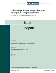
Chapter 2Long-Distance and Rural AreaData SourcesIn the context of statewide forecasting, rural trip-making and long-distance intercity travelconstitute important market segments. Information describing these markets and how they varyfrom state to state has historically been sparse, and many states do not have the resources toinitiate original data collection to develop a set of model parameters. Yet these same states havea pressing need for confidence in reasonable transportation planning results for rural and longdistancetravel. Furthermore, for the states where local data are available, there is little basis toassess how comparable their assumptions are with those from other states.This chapter will address this topic by first identifying differences in rural and urban travelin various states from existing surveys. A high-level analysis of 1995 ATS, 2001 NHTS, 2009NHTS, and select statewide, super-regional, and tourist survey data is provided in this chapter tohighlight how differences in rural and long-distance trip-making occur in different geographicregions and to identify any explanatory variables that could be used to adjust average values andreflect conditions in a particular state. The most recent NHTS contains over 20 separate add-onpartners, some representing full states and some MPO planning areas (which may include ruralareas within the MPO boundary).In conducting analysis, it is important that rural and long-distance data on transferableparameters be compared against urban short-distance data and typical model parameters. Forexample, according to the 2009 NHTS, short trips account for the vast majority of personal tripsin the United States—three-quarters of vehicle trips are less than 10 miles in length. However,these trips account for less than one-third (28.9 percent) of all vehicle miles traveled (VMT).Trips of more than 100 miles account for less than 1 percent of all vehicle trips but 15.5 percentof all household-based vehicle miles, as illustrated in Figure 2.1. With the potential impact onVMT, travel demand forecasts depend on knowing more about the current amount and natureof long-distance and rural travel in the United States.This chapter first assesses national data sources on personal long-distance and rural travel,with a focus on the 1995 ATS, 2001 NHTS, and 2009 NHTS. Long-distance travel includes air,intercity bus and rail, and personal vehicle as the primary modes. There is an acknowledgedlack of sufficient data on long-distance trips, and too little understanding of how travelers makedecisions regarding mode, what kinds of reasons people travel long-distance, and other basiccharacteristics of intercity, interstate, and long-distance travel. Information about surface modes(private vehicle and transit) are particularly important, since for distances less than 500 miles,surface transportation modes move the majority of people.Next, this chapter describes available statewide and regional household travel surveys thatinclude a significant sample of rural and/or long-distance trips. This includes a discussion of theOhio Statewide and Long-Distance Travel Surveys, conducted in 2002–2003, which contacted16,529 households, of which 2,049 made long-distance trips. This is followed by discussion of14

Long-Distance and Rural Area Data Sources 1560504030201001/2 mileor less1/2- 1 mile 1.01-10miles10.01-20miles20.01-30miles30.01-50miles50.01-75miles75.01-100milesmore than100 milesPercent Of TripsPercent Of MilesSource: Author’s analysis of NHTS 2009.Figure 2.1. Vehicle trips and VMT by trip length.the Michigan Travel Counts Study, conducted in 2004 and 2009, with both Michigan effortsincluding a retrospective component focused on trips of 100 miles or greater and sampling areasfor rural travel. Following these main studies, the chapter includes details about other possiblesources of rural or long-distance travel data, from recent and ongoing statewide and global positioningsystem (GPS) surveys to other superregional travel surveys and tourism surveys.2.1 National Travel SurveysThis section provides an overview of the 1995 ATS, 2001 NHTS, and 2009 NHTS. Althoughthe NHTS Add-On components are largely equivalent to statewide surveys discussed in the nextsection, these are still part of the national survey and use the same survey instrument and samplingplans.American Travel Survey (ATS)Overview: The ATS was a national survey of long-distance trips defined as 100 miles or more,one-way. Although over 15 years old, the 1995 ATS remains the primary source of informationat the national, state, and metropolitan-area level about the amount and characteristics of longdistancetravel flows between states and large metro areas.Sample Detail: Sample selection for the ATS was based on households that had participated inthe Current Population Survey (CPS) (http://www.bls.gov/cps/). The sample was based on PrimarySampling Units (PSU) (Lapham, undated), as defined below, and a selection of addresseswithin each PSU. The sample was distributed rather evenly across the states (a choice that generatedsome discussion) to ensure representation from each state. The sample for each statewas designed to include two or more PSUs. All the PSUs were in urbanized areas, so no ruralhouseholds are represented in the dataset. The person trip file contains 116,176 individuals whoreported 556,026 long-distance trips during the survey year. “A trip is defined as each time aperson goes to a place at least 100 miles away from home and returns.”PSUs are small geographic areas carefully selected to represent larger geographic areas. ThePSUs were grouped into two strata; self-representing areas and nonself-representing areas. Selfrepresentingareas generally consist of a single PSU used to represent an entire metropolitan area.The remaining areas, called nonself-representing, were formed by combining PSUs that possesssimilar characteristics, such as geographic region, population density, population growth rate,

16 Long-Distance and Rural Travel Transferable Parameters for Statewide Travel Forecasting Modelsand proportion of nonwhite population, as stated in the ATS overview document. A sample ofnonself-representing PSUs was selected to represent all of the PSUs in the stratum. A total of 729PSUs were sampled—314 self-representing and 415 nonself-representing.Survey Conduct: The households sampled in each of the PSUs were contacted four times, onceeach quarter, to report long-distance travel by the household members. If for some reason thehousehold was not contacted during a quarter, when contact was next made information aboutthe missing quarter was obtained. People who moved out or into the sample household wereretained through recall and imputation. Since the sample was based on addresses, if new peoplemoved into the household, the household remained part of the sample, and retrospective dataabout long-distance travel was collected from the new household members and used in imputationand weighting.The study approach included use of a survey package mailed out to the household with a postcard reminder. The retired CPS households that had telephone numbers on record were interviewedvia computer-assisted telephone interview (CATI) while the rest were interviewed usingcomputer-assisted personal interview (CAPI) and in-person visits (approximately 55 percentCATI and 45 percent CAPI).Limitations of the ATS: The biggest concern with using the ATS is obviously the age of the data,now more than 15 years old. In the intervening decade and a half, major changes have occurredin economics and demographics, communication technology, and security precautions at airports,just to name a few.In addition, the limitations of the survey to trips 100 miles or more one-way might impactassessing the full continuum of travel through the travel demand forecasting process. In theNHTS data series, 30 percent of long-distance trips were in a midrange distance, between 50 and100 miles one-way, and these trips are underreported in the daily estimates of travel. Trips of thisdistance are important to many corridor analyses, but would be missing from the ATS. The lackof rural households (HHs) could be another limitation, especially if it is found elsewhere thatrural HHs make more long-distance trips.Uses of the ATS: The ATS was designed to be useful for multistate and corridor planning andresearch. The large sample size and representation from each of the states means that these datacan be used to estimate state-to-state flows and even some flows between large metropolitanareas if the resulting margin of error (up to 20 percent) can be tolerated, a unique characteristicof the ATS. (Note that the margin of error can be calculated at the state-level based on existingreports, but data for recalculating new margins of error are not available.)The long-range trips captured in the ATS have a significant non-auto mode share, anotherunique characteristic, and separate detail about recurring trips such as long commutes and weekendtrips to second homes. In addition, intermodal connections are captured, allowing analysisof access modes to airports, intercity rail, and intercity bus stations.In 1995, FHWA also conducted one of the national household surveys (then called NationalPersonal Travel Survey), which also had a long-distance component (measuring trips of 75 milesor more taken within a 2-week period). After the release of the 1995 ATS and the 1995 NPTS,there was quite a bit of research to see if the surveys could be combined.A number of similarities and dissimilarities were noted between the two data sources. Forinstance, the ATS was conducted using a panel, where the same household’s reports for eachquarter were used. On the other hand, the 1995 NPTS asked randomly selected households toreport long-distance trips for just the 2 weeks prior to the assigned travel day. The short recallperiod, it was found, is more likely to miss infrequent travelers and perhaps overcount frequent

Long-Distance and Rural Area Data Sources 17travelers. ATS calculated trip distance based on trip origin (zip code centroid), trip destination,and mode used using a national network of highways and air routes. In 1995, the long-distancecomponent of the NPTS calculated distance on the great circle distance of MSA centroid to MSAcentroid, a less precise measure than one that uses network distance.With these and other relevant differences in mind, the two surveys were combined into asingle sample in the 2001 NHTS.2001 National Household Travel SurveyOverview: The 2001 NHTS combined elements of the 1995 ATS and the 1995 NPTS into asingle survey. The survey was designed to obtain trips to destinations 50 miles or more from homewithin the 4 weeks previous to the assigned travel day. The long-distance component was includedin the national sample of 26,000 households, which included 60,000 people. In addition, the Add-On states of New York, Texas, and Wisconsin purchased a long-distance component along withthe daily Add-On.Sample Detail: The NHTS sample was a list-assisted random digit dialing (RDD) telephonesample, which means it consisted of randomly selected telephone numbers matched againstknown lists of commercial and nonworking numbers to maximize the “hit” rate of a workingresidential number. Numbers were only selected from working 100 blocks where at least twoother numbers in the 100 block were assigned. This sample frame was updated quarterly toinclude newly assigned numbers on a regular basis.The drawbacks of a telephone sample include the lower response rates (40 percent in NHTS2001 compared to over 80 percent in 1995 ATS) and the lack of representation of very lowincomehouseholds that might not have telephones. On the plus side, the geographic representationof the sample is much more widely spread, including households in all areas of the countryweighted to Census division.Survey Conduct: The NHTS sampled telephone numbers were preassigned a day of the weekas a travel day, with the travel period being the 4 weeks previous to the travel day, so the travelperiod covers all days of the year. The selected household was sent a precontact letter with anincentive and then called and recruited into the survey. A packet of information was sent to thehousehold with a second incentive. In this packet was a memory jogger for trip reporting (traveldiary) and a map with the household location geocoded (from the address) with a 50-mile circledrawn around it and a reminder to respondents to keep track of any trips to places outside thecircle. The data were collected via CATI.Limitations of the 2001 NHTS: The goal of the long-distance component of the 2001 NHTSwas to provide national-level statistics on basic parameters of long-distance travel, such as frequencyof trips by mode and purpose. Analysis of the recall period of 28 days prior to the travelday shows lower-than-expected trip reporting for air and other trips not in private vehicles, whencompared to the ATS. For example, the 1995 ATS had 18.02 percent of trips reported by air, whilethe NHTS had only 9.23 percent mode share for air (of trips 100 miles or more).In addition, because of the short recall period, the unweighted sample size for 2001 NHTSlong-distance is much smaller than the 1995 ATS—the 4-week travel period collected 45,165long-distance trips compared to 550,000 in one year of ATS. Although these 4-week-period tripswere expanded to represent 1 year of travel, the small sample limits the power of the data atanything less than a national overview.Uses of the 2001 NHTS: The 2001 NHTS long-distance data has a couple of unique componentsthat might be of interest. First, the data can be used to estimate the amount and type of midrangetrips (less than 100 miles in length), a travel component that can be important to corridor planning.

18 Long-Distance and Rural Travel Transferable Parameters for Statewide Travel Forecasting ModelsWithin this mileage range, where air’s mode share is negligible, information on the amountand type of travel is useful. Second, the 2001 NHTS, because of the lowered mileage threshold,included information about recurring trips, such as long commutes, weekend trips to secondhomes, and medical trips. This is a unique source of data on the type and frequency of recurringlong-distance trips.Comparison of Select 1995 ATS and 2001 NHTS Travel StatisticsOne of the key strategies to assess the data sources is to benchmark the estimated travelparameters against each other. Table 2.1 shows some of the trip-based estimates of travel, suchas mode, purpose, and trip length, from the 1995 ATS and the 2001 NHTS. In an effort to maximizeconsistency of results, a mileage threshold of 100 miles was used for analyzing both surveys,even though the NHTS generally used a threshold of 50 miles or more to define long-distanceTable 2.1. Preliminary comparative statistics from ATS and NHTS.Parameter Summary1995 ATSMore Than 100 Miles2001 NHTSMore Than 100 Miles aPercent of Trips by ModePrivate Vehicle 78.51 87.13Air 18.02 9.23Other 3.47 3.64Percent of Trips by PurposeBusiness and Bus/Pleasure 22.42 25.69Visit Friends/Relatives 32.58 26.31Leisure 30.53 26.21Personal/Family or Medical 11.93 9.56Other 2.54 12.22Overall Mean Trip Length in Miles411.88 457.57(One-Way All Modes) bMean Trip Length – Air 1,003.21 2,088.78 cMean Trip Length – Private Vehicle 276.53 301.54Mean Trip Length – All Other 404.02 482.02Mean Trip Length by Purpose in Miles(One-Way All Modes)Business and Bus/Pleasure 467.89 480.93Visit Friends/Relatives 398.77 478.60Leisure 406.70 516.44Personal/Family or Medical 376.05 409.80Other 316.03 276.28Overall Travel Party Size3.10 N/A(All Modes)Travel Party Size – Air 2.98 N/ATravel Party Size – Private Vehicle 2.42 N/ATravel Party Size – All Other 9.34 N/ATravel Party Size by PurposeBusiness and Bus/Pleasure 2.12 N/AVisit Friends/Relatives 2.81 N/ALeisure 3.93 N/APersonal/Family or Medical 2.91 N/AOther 6.34 N/Aa NHTS 2001 includes trips of 50 miles and more. For this analysis only trips of 100 miles andlonger one-way were included.b 1995 ATS “Round-Trip Distance” was divided in half to provide one-way estimates.c NHTS Trip Distance includes extreme values. Trip length was capped at the 99th percentile(5,252.18 miles).

Long-Distance and Rural Area Data Sources 19trips. Analysis of these parameters from the 1995 ATS and 2001 NHTS datasets results in similarestimates at the national level. Primary differences appear in the mode split, where the proportionof air travel is very different, and the mean trip length for air, potentially impacted by 9/11.Travel party size was included in this table, although this statistic could only be calculated for theATS. For the auto mode, this measurement would essentially represent an auto occupancy rate.Further analysis—at a smaller geography, for household-based estimates, or to estimate travel fordifferent demographic groups—may reveal greater dissimilarities between the ATS and NHTS.The two surveys were also investigated for estimating trip generation rates. A key issue to considerin this regard is the timeframe for consideration. Since few households make over 100-miletrips on a daily basis, it was decided to look at such trips on an annual basis instead. Using thistimeframe, the ATS indicates aggregate trip rates of 7.00 trips per household and 4.79 trips perperson (18 years of age and older). More complete listings of potentially transferable parametersare provided in subsequent chapters of this report.2009 National Household Travel SurveyOne of the important characteristics for rural travel parameters is transferability across geographies.The 2009 NHTS is an interesting source of data for rural travel parameters because itincludes rural samples from all over the nation. (The NHTS uses the Census definition of “rural,”that is any census block or block group outside of an urbanized area or urban cluster; on the 2009NHTS the Census 2000 delineation is coded.) This makes it possible to compare householdbasedtravel parameters between urban and rural households, which could start to inform theunderstanding about geographic differences in travel for the same demographic categories ofhouseholds or persons.Urban household travel behavior can differ between different areas of the country (e.g., betweenhouseholds in the Northeast and households in the West). One can expect that rural householdtravel might likewise not be homogeneous, but would vary across locations as well as betweensocioeconomic classes.Table 2.2 shows the sample distribution of all rural households in the 2009 NHTS. A total of43,583 households in rural areas completed the survey. Figure 2.2 shows a map of the Censusdivisions and their constituent states.The distribution is uneven across Census divisions because of the participation of the Add-Ons. The South Atlantic division has so many samples because nearly every state in the divisionincluded an Add-On (Florida, Georgia, South Carolina, North Carolina, and Virginia) and allhad large samples that included rural areas. The other Census divisions are represented by onlyTable 2.2. NHTS 2009 sample of rural households.ItemRural Samples aAll Rural (National) 43,583New England 1,560Mid-Atlantic 5,721East North Central 2,355West North Central 2,684South Atlantic 19,293East South Central 1,570West South Central 6,228Mountain 1,727Pacific 2,445a Includes Add-On samples.

20 Long-Distance and Rural Travel Transferable Parameters for Statewide Travel Forecasting ModelsSource: http://www.census.gov/geo/www/us_regdiv.pdfFigure 2.2. Census regions and divisions.one or two Add-Ons, such as West North Central, which includes the Add-Ons in South Dakotaand Iowa, or East North Central, which includes the Add-Ons in Wisconsin and Indiana. Otherdivisions, such as Pacific, have only one Add-On, in this case the large sample in California.Table 2.3 and Figure 2.3 compare a few important travel estimates from the national samplefor urban and rural households and the same estimates for each Census division. For the purposesof this analysis, rural trips were those that begin and/or end in rural areas.Table 2.3. Travel parameters for urban and rural households by Censusdivision, 2009 NHTS.Person Tripsper PersonAverage VehicleTrip Length (Miles)VMTper HouseholdVMTper PersonUrban Rural Urban Rural Urban Rural Urban RuralAll 3.8 3.6 8.0 12.0 43.5 72.1 17.6 27.4New England 3.8 3.9 9.0 11.7 47.7 79.5 19.9 29.8Mid-Atlantic 3.8 3.7 7.7 11.6 35.6 70.9 14.3 26.9East North Central 4.0 3.6 7.7 11.8 43.2 75.9 18.3 28.6West North4.1 3.6 8.2 10.6 48.3 63.2 21.5 25.3CentralSouth Atlantic 3.7 3.6 8.3 12.6 44.4 72.0 18.5 27.8East South Central 3.8 3.4 8.7 13.3 46.7 75.0 20.7 29.1West South Central 3.8 3.7 8.2 12.3 47.0 72.6 18.6 26.3Mountain 4.0 3.8 7.6 12.0 46.0 76.6 18.3 28.5Pacific 3.8 3.7 7.4 10.6 42.1 64.6 15.6 24.1Source: Author’s analysis of 2009 NHTS, includes travel on weekends and holidays.

Long-Distance and Rural Area Data Sources 21Vehicle Miles (VMT) per day35302520151050AllNewEnglandMidAtlanticEast NorthCentralWest NorthCentralSouthAtlanticEast SouthCentralWest SouthCentralMountainPacificUrbanRuralSource:Author’s analysis of 2009 NHTS, includes travel on weekends and holidays.Figure 2.3. VMT per person for urban and rural households by Census division.As Table 2.3 shows, the number of person trips per person does not vary much between urbanand rural households. Overall, people in urban households make on average 3.8 trips per day,compared to people in rural households who make 3.6. These per capita estimates include peoplewho reported travel and people who did not, by all modes and for all purposes, and across alldays, including weekends and holidays. In developing final travel parameters for rural traveldemand estimation and forecasting, weekday-only estimates will be preferable.However, estimates of vehicle travel, such as vehicle trip length and VMT per household, varyquite a bit more between urban and rural areas. The average vehicle trip length for urban householdsis 8 miles compared to 12 for rural households (50 percent farther). As a result, overallvehicle miles of travel per capita in urban areas is 17.6 miles on average compared to 27.4 forpeople in rural areas (including people ages 5 and older).There are differences in these major estimates between regions of the country for both urbanand rural households. For instance, VMT per person is lowest for households in the Pacific divisionrural areas (24.1 miles per day), and almost 25 percent higher per household for rural areasin New England (29.8 miles per day). This analysis is preliminary, and the apparent differencesin travel demand across geography may disappear when normalized for household size, numberof vehicles, and other traditional cross-classifications, or they may not.Although each state Add-On had a separate sampling scheme, they all included ruralhouseholds, either as a distinct sample strata (such as in Florida) or as part of a populationproportionatesample (such as Texas and California). Figure 2.4 shows a map of the stateAdd-Ons to the 2009 NHTS. Table 2.4 shows the number of rural households sampled andweighted for each of the state Add-Ons. Remember that the sum of all rural households inthe 2009 NHTS is 43,583 of which 39,739 are from Add-On states and the remainder are partof the national sample in non-Add-On states.Table 2.5 shows the same comparative travel characteristics (VMT per household, VMT perperson, average vehicle trip length and person trips per person) for urban and rural householdsin the 15 Add-On states. As with the national and Census division comparisons, large differenceswere not observed across estimates of the person trips per household between rural and urban orbetween state Add-Ons—in fact, they all round to four, except for rural areas in Wisconsin. Butvehicle travel estimates are very different. For example, the average vehicle trip length in ruralareas in Georgia is 14 miles, the highest of all rural estimates of vehicle trip length, compared toits neighbors of Florida and South Carolina, with averages of 11.7 and 11.8, respectively. Notethat all three of these states are in the same Census division of South Atlantic.

22 Long-Distance and Rural Travel Transferable Parameters for Statewide Travel Forecasting ModelsSouth DakotaWisconsinVermontNew YorkIowaCaliforniaIndianaVirginiaArizonaTennesseeNorth CarolinaGeorgiaSouth CarolinaTexasFloridaFigure 2.4. 2009 NHTS state Add-Ons.Table 2.4. Sampled and weighted number of rural households in the 2009NHTS Add-On states.StateSample Size(Rural Households)WeightedHouseholdsWeightedPersonsArizona 1,163 422,238 1,248,929California 2,148 958,264 2,718,128Florida 3,251 1,057,714 2,771,537Georgia 3,569 1,136,647 3,016,386Iowa 1,359 509,618 1,276,488Indiana 1,133 674,247 1,796,446North Carolina 4,664 1,478,175 3,742,939New York 5,452 1,100,822 2,911,999South Carolina 1,974 671,261 1,731,758South Dakota 654 162,405 387,506Tennessee 1,114 897,829 2,378,480Texas 5,902 1,610,731 4,572,820Virginia 5,551 838,240 2,147,874Vermont 1,137 153,587 382,281Wisconsin 668 753,627 1,884,870Sum of All Add-Ons 39,739 12,425,406 32,968,440

Long-Distance and Rural Area Data Sources 23Table 2.5. Travel parameters for urban and rural households by Add-Onstate, 2009 NHTS.Person Tripsper PersonAverage VehicleTrip Length (Miles)VMTper HouseholdVMTper PersonUrban Rural Urban Rural Urban Rural Urban RuralArizona 3.9 3.8 8.5 11.0 49.2 78.4 19.2 26.5California 3.8 3.5 7.6 11.7 44.0 71.0 15.7 25.0Florida 3.6 3.7 7.7 11.7 41.0 68.6 17.1 26.2Georgia 3.7 3.5 8.8 14.0 48.8 83.0 19.2 31.3Iowa 4.1 3.7 6.5 9.7 34.8 57.2 16.1 22.9Indiana 3.7 3.6 7.2 11.1 38.2 70.8 16.7 26.6North Carolina 3.8 3.6 8.6 11.3 45.6 63.9 20.0 25.2New York 3.7 3.5 6.3 10.5 24.0 60.3 9.4 22.8South Carolina 3.9 3.6 8.2 11.8 47.1 69.3 19.8 26.9South Dakota 4.1 3.8 7.1 10.8 43.6 58.2 19.2 24.4Tennessee 3.7 3.5 9.1 11.7 49.2 70.3 22.1 26.5Texas 3.8 3.5 8.5 12.1 48.9 74.1 18.8 26.1Virginia 3.8 3.5 8.0 12.4 43.5 72.5 18.1 28.3Vermont 3.9 3.6 7.3 10.4 38.2 59.3 17.8 23.8Wisconsin 4.0 3.3 7.8 11.9 42.7 62.5 18.9 25.0Average 3.83 3.58 7.81 11.47 42.59 67.96 17.87 25.83Source: Author’s analysis of NHTS 2009, includes travel on weekends and holidays.Analysis of the Florida 2009 NHTS Add-On surveys, conducted for the Florida DOT (FloridaDepartment of Transportation and Cambridge Systematics, Inc., 2010), indicated a significantdifference in average trip length when comparing mean values for urban and rural households.Preliminary analysis of the 2009 Florida Add-On found the average trip length for home-basedwork (HBW) trips to be 25.7 minutes in urban settings and 29.6 minutes for rural households.Average trip lengths provided elsewhere in this report from the 2009 NHTS national sample wereonly provided in miles traveled for all trip purposes.2.2 Statewide Household Travel SurveysThe Ohio and Michigan Departments of Transportation (DOTs) have made significant investmentsin the documentation of demographic and travel behavior characteristics of those residingin the state. This has included statewide household travel surveys with a sizeable sample ofrural residents. The Ohio and Michigan DOTs also conducted long-distance household travelsurveys, with some overlap in households that completed both surveys. Recent and ongoingstatewide household surveys for California, Oregon, and Utah are described in a later section ofthis chapter due to their recent nature.Ohio Statewide Household Travel SurveyThe Ohio Statewide Household Travel Survey was conducted from 2001 to 2003. Sponsoredby the Ohio DOT, the purpose of this survey was to document statewide and regional travelpatterns in order to update travel demand models. (Unless otherwise noted, the details inthis section are from NuStats, Technical Memorandum: 2002–2003 Ohio Statewide HouseholdTravel Survey, prepared for the Ohio Department of Transportation, August 2004.) A total of

24 Long-Distance and Rural Travel Transferable Parameters for Statewide Travel Forecasting Models16,112 households were surveyed, of which 2,530 households are located in rural Ohio, definedas outside an MPO area. The survey was conducted using state-of-the-practice methods, includingrecruiting households to participate, mailing travel diaries to them, and retrieving the traveldetails by phone or mail.All members of participating households reported travel for either a 24- or 48-hour period.Travel days covered all seven days of the week, and travel days were assigned throughout thefall and spring periods, except for weekdays immediately preceding or following a holiday. Thesurvey documented the following data elements:• Household Demographics—Household size, household vehicles, dwelling type, home ownership,home location, and income;• Person Demographics—Age, gender, relationship, licensed driver status, employment status,work location and other work-related details, student status, and school type and location;• Travel Behavior Characteristics—Activity, travel mode, origin and destination of travel (geocodedto x-y coordinates), trip purpose, travel party size and composition, and arrival anddeparture times.The following is a summary of relevant weighted travel statistics obtained overall and for therural households, as documented in the final report for the survey:• The overall average daily trip rates were 7.90 trips per household and 4.94 trips per person. Forthe rural households, these statistics were 7.78 trips per household and 4.79 trips per person.• At the statewide level, trips averaged 18.4 minutes in length. Work trips averaged 20.9 minutesand shopping trips averaged 15.0 minutes. In rural areas, trips averaged 18.8 minutes summedfor all purposes. Work trips averaged 21.0 minutes and those for shopping averaged 16.2 minutesfor rural areas.• Ninety percent of all trips statewide were made by auto (driver or passenger). For the ruralhouseholds, auto accounted for 89 percent of all trips. Figure 2.5 depicts the distribution oftravel by modes statewide and in rural areas.Ohio Statewide Long-Distance Travel SurveyIn 2002, the Ohio DOT embarked on designing and conducting a long-distance travel surveyas a supplement to its statewide household travel survey. (Unless otherwise noted, the details in80%70%60%50%40%68%67%30%20%10%0%23% 23%5% 5%3% 4%1% 1% 1% 0%1% 1%Auto-D Auto-P Car/Vanpool Transit School Bus Walk OtherStatewideRuralSource: NuStats Technical Memo, Ohio Statewide Household Survey, Table 7.7.Figure 2.5. Travel modes from Ohio Statewide Household Survey.

Long-Distance and Rural Area Data Sources 25this section are from NuStats, Technical Memorandum: 2002–2003 Ohio Long-Distance TravelSurvey, prepared for the Ohio Department of Transportation, March 2005.) Over the 2-yearstudy period, long-distance travel data were obtained from more than 8,000 households acrossthe state, of which 6,113 were summarized in the report. For this study, a long-distance trip wasdefined as a nonwork trip of 40 miles or longer. (In Appendix E of the NuStats report, the CATIsurvey question LDQ1 asks about travel 50 miles or more away from home.) The long-distancesurvey asked respondents to list any trips over 40 miles, even though over 50 miles is the longdistancethreshold defined in the model. The lower 40-mile threshold was used in the survey realizingthat respondents might leave out valid over 50 trips with a 50-mile survey cut-off. Reportedtrips between 40 and 50 miles were later excluded during model development.There were three approaches used in collecting the data: a 2-week retrospective survey administeredto households that were participating in the statewide household travel survey; a 2-weekretrospective survey administered to randomly sampled households not participating in the statewidehousehold travel survey; and a 4-week prospective survey of nonhousehold travel survey householdsthat were prescreened and identified as having a probability of making a long-distance trip.Long-distance travel was documented for all household members, regardless of age for the specifiedtime period. Trips were recorded regardless of the day of week (i.e., weekday or weekend). However,trips were not recorded during the summer or during a week where a holiday was observed.The survey documented the following data elements:• Household Demographics—Household size, household vehicles, dwelling type, home ownership,home location, and income;• Person Demographics—Age, relationship, employment status, work location, worker occupationand industry, student status, and school type and location; and• Travel Behavior Characteristics—Number of noncommute long-distance trips, destinationof travel, trip purpose, mode of travel, travel party size, and intermediate stops.The resulting Technical Memorandum summarized key statistics obtained from this surveyfor households completing the 2-week retrospective surveys (both those linked to the statewidehousehold travel survey as well as those that were not). (The Ohio DOT has provided accessto the full dataset for use in this analysis.) The overall trip rate was 6.44 for nonwork longdistancehousehold trips per 2-week nonholiday and nonsummer period. More than one-third(37 percent) of the 2.5 million Ohio households reported some level of long-distance trips.As shown in Figure 2.6, households from Akron, Dayton, and Springfield were more likely to16%15%15%14%13%12%10%8%6%6%8%9%10%9%10%6%4%2%0%Toledo(TMACOG)Lima(LACRPC)Dayton(MV)RPCSpringfield(CCSTS)Akron(AMATS)Canton(SCATS)Mansfield(RCRPC)Source: NuStats Technical Memo, Ohio Statewide Long-Distance Travel Survey, Table F.2.Steubenville(BHJTS)Youngstown(EDATS)Figure 2.6. Geographic distribution of households reporting long-distancetravel from Ohio Long-Distance Travel Survey over 2 weeks.Rural

26 Long-Distance and Rural Travel Transferable Parameters for Statewide Travel Forecasting Models70%60%63%50%40%30%20%10%5%12%9%2%1%3%3%3%0%0%0%0 1 2 3 4 5 6 7 8 9 10+Source: NuStats Technical Memo, Ohio Statewide Long-Distance Travel Survey, Table F.28.Figure 2.7. Number of long-distance travel trips reported per household fromOhio Long-Distance Travel Survey over 2 weeks.report long-distance travel as compared to those from other parts of the state. This is due to theirproximity to a larger urbanized area.The majority of households (63 percent) reported no long-distance trip-making during the2-week reference period, as indicated in Figure 2.7. The vast majority of long-distance trips(92 percent) were made by auto, either driver or passenger. As depicted in Figure 2.8, travel byair was a distant second at 5 percent of long-distance trips reported.An important feature of the Ohio survey is that the prescreened prospective sample was onlyused as a way to establish detailed characteristics of long-distance trips for micro-simulationwhile the random retrospective sampling established tour rates. This survey design allowed forobtaining adequate samples for micro-simulation even though the prospective sample is obviouslybiased to households likely to make such trips.Michigan Statewide Household Travel SurveysIn 2004, Michigan DOT undertook an extensive survey of 14,280 Michigan households(http://www.michigan.gov/documents/MDOT_TravCharTR_Final20060804_167340_7.pdf).1% 5% 1%Auto or van or truck driverAuto or van or truck passenger40%52%Bus (public transit)Commercial airplaneOther, specifySource: NuStats Technical Memo, Ohio Statewide Long-Distance Travel Survey, Table 7.29.Figure 2.8. Long-distance trip travel modes from Ohio Long-DistanceTravel Survey.

Long-Distance and Rural Area Data Sources 27The survey documented basic demographics and 48 hours of weekday travel information for allhousehold members regardless of age. For sampling purposes, the state was divided into sevengeographic areas, including three rural areas: southern lower peninsula rural (2,059 households),northern lower peninsula rural (2,073 households), and upper peninsula rural (2,027 households).A second round of household surveys was conducted in 2009.The survey documented the following data elements (http://www.michigan.gov/documents/MDOT_travelcounts_results_Appendices_20_to_24_142289_7.pdf.):• Household Demographics—Household size, household vehicles, household workers, homelocation, and income;• Person Demographics—Gender, age, relationship, driver’s license status, transit pass status(and if one is held, what type and cost), educational attainment, student status, school typeand location, employment status, industry, and work location; and• Travel Behavior Characteristics—Origin and destination of travel, activities at origin anddestination, travel mode(s), travel party (if travel by auto), and parking cost.The following is a summary of relevant travel statistics obtained statewide and for the ruralhouseholds, as readily available in the final report for the survey.• The overall average weekday 48-hour person trip rates were 17.3 trips per household and 6.9 tripsper person. In the southern lower peninsula rural area, the 48-hour statistics were 17.1 trips perhousehold and 6.7 trips per person. In the northern lower peninsula rural area, the statisticswere 15.5 trips per household and 6.3 trips per person. For households in the upper peninsularural area, the average 48-hour trip rates were 16.0 trips per household and 6.7 trips per person.• Average daily household trip rates were estimated at 8.70 trips per household, statewide. Incontrast, the average daily trip rates for the three rural areas were 8.54 trips per household in thesouthern lower peninsula rural area, 7.75 trips per household in the northern lower peninsularural area, and 8.00 trips per household in the upper peninsula rural area.Michigan Statewide Long-Distance Travel SurveysBoth the 2004 and 2009 MDOT “Travel Counts” statewide travel survey efforts included along-distance travel survey component, in which long-distance trips were defined as any trip ofmore than 100 miles away from home that occurred in the 3 months prior to the survey.In terms of the data collection approach, the long-distance supplemental questions wereprinted directly into the travel log, with the instructions to “please provide the following informationfor ALL trips you took within the last 3 months, greater than 100 miles (one-way) fromhome” (http://www.michigan.gov/documents/mdot/mdot_MTC_II_appendices_333723_7.pdf). By including the questions in the travel log, long-distance travel was requested for allhousehold members, regardless of age for the specified time period. In the first effort, traveldiary data were recorded from April 4 to June 10, 2004, then again from September throughDecember 2004 (http://www.michigan.gov/documents/MDOT_travelcounts_results_Final_Report_142283_7.pdf). In the second effort, travel was recorded September through December2009, so long-distance data reflects late summer and fall of 2009.In both efforts, the survey documented the following data elements:• Household Demographics (through the household travel survey component)—Householdsize, household vehicles, household workers, home location, and income;• Person Demographics (through the household travel survey component)—Gender, age, relationship,driver’s license status, transit pass status (and if one is held, what type and cost),educational attainment, student status, school type and location, employment status, industry,and work location;

28 Long-Distance and Rural Travel Transferable Parameters for Statewide Travel Forecasting ModelsTable 2.6. Michigan travel counts long-distance trip rates.2004 Survey 2009 SurveyNumber of Households 14,818 a 1,975Number of Long-Distance Trips 37,338 4,567Household Trip Rate (3-Month Period) 2.18 2.31Household Annual Trip Rate 7.34 6.25Source: Abt SRBI Comparison Report, Michigan Travel Counts Survey, Table 5.16.a The difference in number of households in the 2004 survey reflects initial results (14,818) versusresults after additional data cleaning (14,280).• Travel Behavior Characteristics—Origin and destination of travel, activities at origin anddestination, travel mode(s), travel party (if travel by auto), and parking cost; and• Long-Distance Travel Behavior Characteristics—Destination (city and state or country ifinternational), day of departure and day of return, primary reason for trip, primary mode todestination and transportation used at destination, and the number of times this specific tripwas made during the 3-month period and the past 12 months.A total of 14,280 households from across the state were surveyed in the 2004 effort, with eachmember of the household completing a 24-hour travel diary. Both diaries included the longdistance3-month retrospective log at the front of the diary. Table 2.6 summarizes the number ofsurveys, reported trips, and estimated long-distance trip rates resulting from each survey effort.The documentation of long-distance travel is more extensive in the 2004 survey comparedto what is available for the 2009 survey. Figure 2.9 presents 2004 survey findings with respect tolong-distance travel. In terms of trip purpose, the majority of long-distance trips were reportedfor pleasure (63 percent), followed by trips for personal business (18 percent) and business purposes(15 percent).The majority of long-distance trips were made by private auto (87 percent), as depicted inFigure 2.10. Air travel accounted for 10 percent of the trips, while bus and train accounted forvery small proportions of the long-distance travel. (Note that for business trips, airplane travelaccounts for 23 percent of all trips.)2.8% 1.8%14.8%17.7%BusinessPleasurePersonal BusinessSchool/ChurchOther62.9%Source: Michigan DOT Travel Characteristics Technical Report, Figure 45.Figure 2.9. Michigan travel counts, long-distance trippurpose.

Long-Distance and Rural Area Data Sources 291.1%10.2%0.4% 1.7%Private vehicleAirplaneBusTrainOther86.6%Source: Michigan DOT Travel Characteristics Technical Report, Figure 46.Figure 2.10. Michigan travel counts, long-distancetravel mode.Other pertinent findings from the 2004 Michigan long-distance surveys include• The majority of long-distance trips (60 percent) are to destinations within the state, and• In rural areas, most long-distance trips are for personal business. According to the MichiganDOT, this “indicates that the services available from trade centers within 100 miles of theselocations lack amenities available” in the larger cities.Although trip distances were not provided in the summary data, the Michigan DOT didinclude a map summarizing the proportion of long-distance trips to different areas of the UnitedStates. This map, see Figure 2.11, shows that most trips are to surrounding areas in state andin neighboring states, with the exception of Florida attracting a large number of Michigan“snowbirds” and tourists.2.3 Supplemental Sources of Rural and Long-Distance DataIn addition to the surveys discussed above, there are other survey sources that could be usefulin developing the rural and long-distance transferable parameters. These sources are consideredsecondary because they are (1) recently completed and without complete documentation,(2) currently being fielded and thus unavailable, or (3) require data mining to obtain usefulresults for this study. These include• Front Range Travel Counts Long-Distance Survey (Colorado),• California Statewide Travel Survey,• Oregon Household and Activity Survey, and• Tourism surveys.For these secondary travel surveys, the travel survey team either recently completed datacollection (so the data would be available to inform this study but a report with results has notyet been issued), collected relevant data as a naturally occurring event during the travel diaryperiod but did not analyze it separately (so the data would be available to inform this study butwill require some mining efforts), or knows currently travel surveys are being conducted thatdocument the needed data (so the data would be available at some point to inform future studies).Similarly, tourism surveys are usually conducted for economic development purposes, but containsome O/D detail. They are summarized here because the data may be useful in estimating therelative attractiveness of certain areas over others for long-distance travel in particular.

30 Long-Distance and Rural Travel Transferable Parameters for Statewide Travel Forecasting ModelsSource: Michigan DOT Travel Characteristics Technical Report, Figure 44.Figure 2.11. Michigan travel counts, long-distance trip destinations.Front Range Travel Counts Long-Distance SurveyThe Front Range Travel Counts Survey (FRTC) is a comprehensive study of the demographic andtravel behavior characteristics of Colorado Front Range residents across four MPO regions: NorthFront Range (Fort Collins), Denver, Colorado Springs, and Pueblo, as depicted in Figure 2.12. Theobjective of the survey effort is to document demographic and travel behavior characteristics acrossthe Front Range in order to support travel demand modeling and answer travel-related questions.As part of the FRTC, a household travel survey was conducted in all four MPO regions. Inaddition, surveys were conducted to obtain data regarding commercial travel, travel into andout of the region, and residential travel that was more than 50 miles in distance. Data collectionfor the effort was conducted from 2009 to 2011. At the time of this report, the project was in thepost-collection data processing stage.As indicated in Figure 2.12, the study area includes metropolitan Denver, but also the smallerurban and rural communities along the I-25 corridor. A total of 12,415 regional households completedthe 24-hour diary study. When analyzed, the geographic diversity will help to documentdifferences in travel for rural versus nonrural households. In addition, within the household travelsurvey design, respondents were instructed to report all trips within the study area. Of more than115,000 trips in the cleaning stage, approximately 889 trips are preliminarily flagged as being50 miles or longer one-way. Of these 889 long-distance trips, one-fourth reflect a work commute.Given the expectation that long-distance travel would be a relatively rare event, a long-distancesurvey was added as a supplement to the household travel survey in order to document residentialtravel more than 50 miles in distance. This supplemental survey was conducted in two stages.First, for all households where data collection had been completed and the household indicatedan interest in participating in follow-up studies, the household was mailed a long-distance logand asked to record all travel 50 miles or longer for noncommute purposes made by the household

Long-Distance and Rural Area Data Sources 31Source: NuStats, 2011.Figure 2.12. Front Range study area.members in the 2 weeks prior to a reference date (logic being that the commute trips would becaptured in the 24-hour travel logs while all other long-distance trips were less regular and thusmight not be captured in the 24-hour travel logs). Second, for households in the data collectionstage of the survey, the long-distance log was provided in the same packet as the 24-hour traveldiary and households were asked to record all travel 50 miles or longer that was not a work commutetrip made by household members in the 2 weeks prior to the travel date. For this secondgroup of households, if no long-distance travel was reported, the household was asked for the dateand location of their last trip that met the definition of a long-distance trip.One-fourth (25 percent) of all households reported a long-distance trip, with a total of 8,680 tripsin post-collection processing. This suggests that the unweighted trip rate is approximately 2.77 longdistancetrips per household per 2-week period. These data have not been processed for summarystatistics yet, weighted, or expanded. Comparisons of long-distance trip-making among differenthousehold travel surveys in this report are preliminary and reflect different thresholds for identifyinglong-distance travel.California Statewide Household Travel SurveyThe California DOT (Caltrans) is currently conducting a statewide household travel survey(http://www.scag.ca.gov/modeling/mtf/presentations/012611/mtf012611chts.pdf). The projectedsample size is 60,000 households, with most households completing a 24-hour weekdaydiary but some completing a 48-hour diary to capture weekend travel. The design includes apurposeful oversample of rural areas and a supplemental long-distance survey. When completedin 2012, this will provide a rich source of information for both rural and long-distance research.The last statewide household travel survey in California was conducted in 2000/2001 (http://www.dot.ca.gov/hq/tsip/tab/documents/travelsurveys/2000_Household_Survey.pdf). A total of

32 Long-Distance and Rural Travel Transferable Parameters for Statewide Travel Forecasting Models17,040 households participated in the survey, documenting demographic and travel behaviorcharacteristics in a 24-hour diary study, conducted using state-of-the-practice methods. Dataelements included household size, income, vehicle ownership, employment status of each householdmember, and housing unit type as well as trip times, mode, activity at location, origin anddestination, and vehicle occupancy. As with the Front Range effort, rural areas were surveyedand long-distance travel was obtained as it naturally occurred during the travel period. Thus,with data mining, this older survey may provide insights to aid in the estimation of rural andlong-distance travel parameters.Oregon Household Activity SurveyThe Oregon Household Activity Survey is a statewide effort to document demographic and travelbehavior characteristics of its residents (http://www.oregon.gov/ODOT/TD/TPAU/Survey.shtml).Launched in 2009, the survey will provide insights gleaned from over 17,000 households that areproviding 24-hour travel details for all household members. In terms of documenting rural travel,the sampling plan was designed to cover the entire state, especially the rural areas outside the metropolitanareas in the state as shown in Figure 2.13. In addition, this effort instructs respondents toreport all travel within the State of Oregon, so intercity travel can be captured. The Oregon DOT iscurrently considering a long-distance supplemental survey.Recent Global Positioning System (GPS) SurveysSeveral recent GPS-based household surveys have been analyzed for results relevant to ruraland long-distance travel. Similarities in designs across these studies influence some of the results(e.g., weekend versus weekday proportions). In addition, the studies purposefully assigned the GPSunits to long-distance commuters. The GPS-based survey statistics compiled for this analysis includethe following, along with the breakdown of long-distance, rural, and urban trips for each survey:Source: http://sites.nustats.com/otas/Figure 2.13. Map of Oregon.

Long-Distance and Rural Area Data Sources 33• Atlanta Household Travel Surveys (2011):– 580 long-distance trips (1%);– 16,932 rural trips (26%); and– 48,098 urban trips (73%).• Denver Household Travel Surveys (2010):– 395 long-distance trips (1%);– 9,836 rural trips (24%); and– 31,377 urban trips (75%).• Massachusetts Household Travel Surveys (2010):– 176 long-distance trips (1%);– 3,349 rural trips (24%); and– 10,325 urban trips (75%).• Chicago Household Travel Surveys (2008):– 102 long-distance trips (1%);– 1,572 rural trips (10%); and– 14,032 urban trips (89%).Additional information on these GPS surveys can be obtained at the following web addresses:• Atlanta Regional Commission/Atlanta Household and Activity Travel Survey/2011 (http://www.atlantaregional.com/transportation/travel-demand-model/household-travel-survey).• Denver Regional Council of Governments/Front Range Travel Survey/2010 (http://www.drcog.org/index.cfm?page=RegionalTravelBehaviorInventory).• Massachusetts Department of Transportation/Massachusetts Statewide Household TravelSurvey/2010 (http://sites.nustats.com/travelsurvey/faq).• Chicago Metropolitan Agency for Planning/Travel Tracker household travel survey for Chicago/2008 (http://www.cmap.illinois.gov/travel-tracker-survey).Tourism SurveysSurveys conducted to track tourism visits are another source of data regarding long-distancetravel. These surveys are conducted at state, regional, and location-specific levels, conducted primarilyto inform economic development efforts and fine-tune marketing campaigns. From a travelbehavior point of view, these surveys do not document the key variables necessary to inform thedevelopment of parameters or for use in a model. However, they provide qualitative details that cansuggest attraction rates for existing tourist areas, thereby improving the fit of a long-distance model.Statewide Tourism SurveysTourism can play a large role in some states’ economic budgets. Some states conduct surveys ofvisitors to improve tourist’s needs. Examples of the data available from state surveys that mighthelp with forecasting long-distance travel are shown in Table 2.7. The transferability of suchsurveys, usually collected in high tourism states, should probably be limited to other states witha large tourist component to their economy.Regional Tourism SurveysSome regions conduct surveys of visitors to learn what motivates tourists to visit their attractions.Regional survey findings vary by location. Specific locations obtain different survey results.Each region’s results will determine the type of variables needed to predict future visitor numbers.Results from two regional surveys are shown in Table 2.8.National and State Park SurveysMany national and state parks collect visitor information from patrons using surveys. Theirsurveys are collected routinely with an abundance of data. A majority of the information collectedvaries by park location. Four park survey results are shown in Table 2.9.

Table 2.7. Statewide tourism surveys.Characteristic State of Oregon State of Hawaii State of FloridaData CollectionMethodsUniverse (orSample Size)Data CollectionDurationOnline surveyCombined surveys andstatistics from other sourcesCombined surveys andstatistics from other sources,including international512 (sample) 6,517,054 visitors 80,879,000 visitorsApril 29 toMay 17, 2005Origins California (14%);Oregon (14%);Washington (6%);Florida (4%);Arizona (4%);Pennsylvania (4%)2009 2009Continental U.S., Japan,Canada, Europe, Other;U.S. West – 2,718,818 (by air);U.S. East – 1,561,468 (by air);96,606 (by cruise ship)Canada 2,644,000 (3%);Domestic 71,246,000 (88%);Overseas 6,989,000 (9%)Group Size N/A Average 2.1 Average 2.3 aAge N/A N/A 46 aTravel Mode N/A 6,517,054 visitors arrived by air;96,606 visitors by cruise ship41,509,000 (51.3%) air;39,370,000 (48.7%) non-aira Domestic trips only (auto and air).Table 2.8. Regional tourism surveys.Characteristic Yuma Area, Arizona Cape Cod, MassachusettsData Collection Methods Paper Surveys Online SurveySample Size 1,316 N/AData Collection Duration January 2010 to December 2010 2006Origins One-fourth from Arizona (26.9%),(25.2%) came from California. AfterCalifornia, the other top 10 statesfor domestic visitors wereWashington, Texas, Oregon,Michigan, Illinois, Florida, Nevada,Maryland and Virginia. WithinArizona, Greater Phoenix areaaccounted for 48.1%, 25% were fromPima County. Among foreignvisitors, Canadians accounted for70.3%, United Kingdom provided11.9% of visitors.Group Size Average 2.6;only 9.2% had children under 18Average:Massachusetts (42%),Connecticut (16%), andNew York (10%)Spring 2006 – 49% traveled as acouple; summer 2006 – 31%traveled as a family; fall 2006 –63% traveled as a coupleAge Average 51 years old Average 31-45 years oldTravel ModeStay DurationThree-fourths of visitors to theYuma area (75.5%) traveled in anautomobile – 57.6% in a private carand 17.9% in a rental car; inaddition, 13.2% traveled in aRV/camper, 7.4% by airplane, and2.3% by motorcycleDay visitors spent an average of3.6 hours in the Yuma area whileovernight visitors spent an averageof 2.7 nightsN/ASpring 34% stayed 1-2 days and17% stayed 3-4 days; summer25% were here on a day tripwhile 30% stayed 3-4 days; fall33% were here on a day trip and34% stayed 1-2 days

Long-Distance and Rural Area Data Sources 35Table 2.9. National and state park surveys.CharacteristicGrand CanyonNational ParkPennsylvania –Ohiopyle (SW),Pymatuning (NW),Greenwood Furnace(SC), Parker Dam(NC), Ridley Creek(SE), andLackawanna (NE)Wyoming –Bear River, Boysen,Buffalo Bill, CurtGowdy, EdnessKimball Wilkins,Glendo, Guemsey,Hawk Springs, HotSprings, Keyhole,Medicine Lodge,Seminole, SinksCanyonChickamauga andChattanoogaNational MilitaryPark,Fort Oglethorpe,GeorgiaData CollectionMethodsSample SizeData CollectionDurationIntercept surveys atthe park4,451 surveysreturned (57% rate ofreturn)September 2003 toAugust 2004Who Traveled California (12.2%),Arizona (8.9%),Texas (4.8%),Florida (3.4%), andNew York (3.2%).Foreign origins (17%),United Kingdom(3.8%),Canada (3.5%),Japan (2.1%),Germany (1.9%), andNetherlands (1.2%)Group Size Average 3.4; only 30%had children under 1825- to 35-minuteinterviews at the parkInterviews – every5th vehicle atpark entrancesPostcard interceptsurveys and licensetag O/D1,139 (adults over 18) 3,914 597summer 2008(Memorial Daythrough Labor Day)N/AAverage 5; majorityvisited in groups of1-32009 July 2003Half fromout-of-statePark trips (17%) andcut-through trips(83%)Average 3.14 Average 2.3Age Average 48.5 Mostly between 36-50 Average 36.3 N/AEducation 85.2% some college Advanced education N/ARepeat VisitorsTravel Mode58.6% first time;41.4% repeatPrivate vehicles(59.7%) combinedwith rental vehicles(37.4%) were used by97.1% of respondents.Allowing for multipleresponses,commercial airlines(16.4%) and RVs(7.8%, private andrental).N/A64% previous visitors N/A75% travel with traveltrailer, motor home,or other camping unitAuto (96.7%)(continued on next page)

36 Long-Distance and Rural Travel Transferable Parameters for Statewide Travel Forecasting ModelsTable 2.9. (Continued).CharacteristicGrand CanyonNational ParkPennsylvania –Ohiopyle (SW),Pymatuning (NW),Greenwood Furnace(SC), Parker Dam(NC), Ridley Creek(SE), andLackawanna (NE)Wyoming –Bear River, Boysen,Buffalo Bill, CurtGowdy, EdnessKimball Wilkins,Glendo, Guemsey,Hawk Springs, HotSprings, Keyhole,Medicine Lodge,Seminole, SinksCanyonChickamauga andChattanoogaNational MilitaryPark,Fort Oglethorpe,GeorgiaOriginsTraveling largely inpersonal vehicles,visitors averaged 792miles of driving inArizona, most oftenusing Interstate 40 asa travel corridor(60.1%).Day users, passiverecreationists(picnickers, beach/pool users), lowerincome,and minorityvisitors were morelikely to say that theproximity of thestudy park to theirhome was excellentand were more likelyto visit only that statepark (and visit morefrequently than othergroups).Half from out-ofstate,40% of boaterswere from ColoradoStay Duration N/A Day visitors Overnight visitors(average 45.3 hours)Not reportedN/A

Chapter 3Transferability and TypologiesThis chapter of the Guidebook identifies alternate approaches and contexts to developingparameters that are more fully developed in later chapters. Although some of the suggestions inthis chapter were not feasible to undertake in the final analysis for this study, these are still importantconsiderations should additional analysis be warranted in the future, either at the nationallevel or for the purposes of individual statewide model development efforts.This chapter provides general guidance on when and when not to transfer model parametersby identifying conditions and parameters conducive to transferability, depending on availabledata sources and other considerations, and expanding on discussions about this topic foundelsewhere in this report. This chapter also describes procedures for consideration in conductinganalysis, both for this study and future research by others at the state or regional level. Transferability,analysis procedures, and typology topics covered in this chapter include the following:• Conditions conducive to transferability—Demographic and geographic considerations aswell as availability of local data;• Parameters to be considered for transferability—Which parameters are easiest to estimate andhave sufficient data to support transferability;• Temporal analysis considerations—Daily, monthly, annually, time of day, seasonality, weekdays,weekends, etc.;• Other aspects of “trip” definition—Consideration of intermediate stops, trips versus tours, etc.;• Proposed process to use datasets for developing transferable parameters—Identifying whatmodel parameters can be estimated, where applicable, from these datasets and the level/typeof effort involved;• Limitations of all datasets—Identifying geographic, trip type, or modal limitations in theaccuracy of the data;• Minimum amount of local data required to assess the reasonableness of parameters—Howthe resulting parameters can be tested or compared for reasonableness; and• Long-distance and rural typologies—How to stratify households, trips, and areas.Later chapters of this report quantify some of the general guidance and analysis proceduresprovided in this chapter by model step.3.1 Conditions Conducive to TransferabilityA set of draft rules must be established indicating conditions conducive to transferability andthose that are not. Such considerations will include, but not be limited to, the following:• Population densities;• Median income;37

38 Long-Distance and Rural Travel Transferable Parameters for Statewide Travel Forecasting Models• Available transportation modes;• Key employment types/industries;• Proximity to tourist destinations; and• Source of model parameter.Population density is a potential indicator of model transferability. This is particularly thecase with mode choice for long-distance travel, as private passenger vehicles predominate inlong-distance travel in smaller-sized urbanized areas and rural areas while long-distance travelis more common on alternate modes in large metropolitan areas. Clearly there is a relationshipbetween population density and available transportation modes that also explains the modechoice issue. Density explains some differences in trip rates, trip lengths, and auto occupanciesof urban versus rural trip-makers.With respect to analysis of median income impacts on trip-making, it stands to reason thatlower-income households make fewer long-distance trips than higher-income households. Likewise,household decisions on transportation modes for long-distance travel include an incomecomponent. The Guidebook chapter on trip generation provides additional understanding onthe relationship between income and rural trip-making.Key employment types and industries can impact rural trip-making. A good example of thisis tourism and lodging, which has a large need for low-income workers who cannot afford to livein proximity to resort developments. Such areas are also magnets for long-distance travel sincevisitors to resorts usually reside outside of the region.The source of the model parameter is a key decision point in parameter transferabilitybecause there is a wide variety of sources considered in establishing such settings, including stateDOT surveys (both household and intercept), surveys from adjacent or similar states, nationalsurveys, MPO surveys, NCHRP Report 716 and other model guidance documents, as well asother statewide models. Furthermore, smaller states (e.g., Rhode Island) might have more incommon with urban and regional models than statewide models, with a smaller percentage oflong-distance trip activity and dominated by urbanized land.Clearly, long-distance model parameters should be derived from surveys with a statisticallyvalid sample of such trip-makers. Rural model parameters require a survey with both urbanand rural resident components in order to ensure that the resulting rates are in fact the result ofdifferences in residential and/or work location and not just due to error in survey execution ordesign. Although reported statistics from statewide models and documentation of general guidanceare useful to provide context, such comparisons are no substitution for analysis of travelsurvey data.The limitations of the data sources must also be considered, especially as these relate to geographiclimitations or trip definition. The minimum amount of data needed for the geographyintended (national, regional, state, or metro area) must be assessed for each of the parameters.3.2 Parameters to Be Considered for TransferabilitySome potentially transferable parameters that are important to properly estimating longdistanceand rural travel patterns and comparative benchmark statistics for statewide models aredescribed in this section. Potentially transferable parameters include the following:• Daily (weekday and weekend) rural trip rates per household by household characteristics(e.g., number of workers by industry) and by trip purpose;• Monthly or annual long-distance trip rates per household by household characteristics(e.g., median income) and by type of trip (trip purpose);• Friction factors, gamma functions, or utilities for rural travel by trip purpose;

Transferability and Typologies 39• Friction factors, gamma functions, or utilities for long-distance travel by trip purpose;• Auto occupancy rates for rural vehicle trips by trip purpose; and• Party size for long-distance trips by trip purpose.In addition to the transferable parameters itemized above, and the dynamics noted earlier inthis chapter, reasonableness values are documented in later chapters for the following:• Percent of rural trips by purpose;• Percent of long-distance trips by trip purpose;• Average (mean) vehicle trip length of rural trips by mode and purpose;• Average vehicle trip length of long-distance trips by mode and trip purpose; and• Percent of long-distance and rural trips by mode (private vehicle, rail/bus, air, other) andtravel distance.Other parameters and benchmarks more difficult to quantify, and less likely transferable,include intermodal connections (e.g., dropped off/drive and park at airports); percent of nontravelinghouseholds by type; and percent of trip destinations to locations within the same stateor to another state.3.3 Temporal Analysis Considerations of TransferabilityDefining what constitutes a statewide model trip is also important to a discussion on transferability.Even this varies among different statewide models, with a few that essentially do notinclude intra-urban trips (e.g., Louisiana). Trips could be defined by person, household, or evenvehicle in some cases. Sometimes, it might make sense to include intermediate stops as trip ends;however, this would seemingly go against the concept of long-distance trips. In fact, what travelerstypically think of as a “(round) trip” is what transportation planners consider a “tour.” A few statewidemodels (e.g., Ohio, Oregon, and New Hampshire) use the concept of tours instead of trips.For rural travel analysis, average weekday conditions would likely be preferable. Similarto regional models, while it might be best to exclude travel on weekends and holidays, suchlimitations could result in sample size problems. NHTS staff have indicated that approximately25–30 percent of 2009 NHTS surveys were conducted on weekend travel; however,weekend travel includes Friday after 6:00 p.m. (teleconference with Adella Santos, FHWA;Vidya Mysore and Frank Tabatabaee, Florida DOT; and Rob Schiffer, Cambridge Systematics,Inc. on August 10, 2011), a timeframe that is similar to other weekday evening peak periodsin many regional models. In states with a singular, well-defined peak season, considerationcould be given to only including surveys that constitute peak season average weekday trafficinstead of annual average daily traffic (AADT), although such a timeframe of analysis wouldnot be recommended for a study on national transferability such as this.Conversely, since long-distance travel is not an everyday occurrence in most households,monthly or annual statistics are appropriate for survey analyses. Also, it is essential to includeweekends and holidays in any survey analysis of long-distance travel because these time periodsreflect where the greatest amount of such travel takes place. Consideration was given to developingtime-of-day factors both for rural and long-distance trips during this study; however, withthe infrequency of long-distance trips, use of trip rates by time of day might be overkill.3.4 Other Aspects of Trip Definition for TransferabilityIn addition to temporal considerations, there are other aspects to be considered in defininga trip for the purposes of research and analysis of transferable parameters. The first of these isconsideration of person trip versus vehicle trip analysis. Since the majority of statewide models

40 Long-Distance and Rural Travel Transferable Parameters for Statewide Travel Forecasting Modelsdeal with person trips and starting with vehicle trips almost precludes a mode choice process,transferable parameters in this study are provided for person trips rather than vehicle trips.Long-distance trip-making was considered at 2–3 different thresholds to determine how parametersdiffer at each threshold.Another consideration is how to deal with intermediate stops and whether these should constitutea trip end or not. Clearly, long-distance trips require stops for gas, food, and/or lodging.In the context of a regional model, these intermediate stops for shopping, etc., would each representa unique nonhome-based trip. In the context of most statewide, multistate, or nationalmodeling, however, these intermediate stops are not of tremendous importance in defining andsimulating a trip. On the other hand, it is probably worth considering an intermediate stop atthe end of the day for lodging as the end of a daily trip, assuming the analysis is daily rather thanmonthly or annually. The location of intermediate stops, relative to congestion on Interstate highwaysor crossroads, could result in greater interest about intermediate travel patterns. The numberand duration of stops will also be addressed in this research.The topic of intermediate stops also leads directly to consideration of tours versus trips. Theprevious lodging example might be better addressed as a stop during a tour rather than theendpoint of the trip; however, the majority of statewide models are still trip-based. Thosestatewide models that are tour-based were developed using statewide travel surveys and, as aresult, will not likely have as much use for transferable parameters. However, the preparationof tour-based parameters is beyond the scope of this report. Hence, the number of intermediatestops for long-distance trips is provided later in this Guidebook based on analysis ofthe 1995 ATS.3.5 Process for Developing Transferable ParametersDatasets with the greatest potential for developing transferable parameters for rural travelare the 2009 NHTS and readily available analyses from the Michigan and Ohio statewide travelsurveys. New and ongoing surveys in California, Colorado, Oregon, and Utah could also proveuseful in documenting rural travel patterns. Transferable parameters for long-distance travelare best derived through a combination of the 2001 NHTS, 1995 ATS, and readily availableanalyses from the Michigan and Ohio long-distance travel surveys.The development of transferable parameters from any of these household diary surveysrequires some level of significance testing to identify what comparisons, typologies, geographies,and time periods best explain or influence the characteristics of rural and long-distance travel.The following dynamics must be considered in the analytical process:• Comparisons—Comparisons should include rural versus urban households and longdistancetrips versus routine (urban and rural) travel.• Typologies—Rural and long-distance travel should be analyzed by household characteristicssuch as income, number of workers, household size, auto availability, etc. “Type” or purposefor long-distance trips can be equated to ATS categories of business, pleasure, and personalbusiness while rural trips can be described using typical home-based and nonhome-basedpurposes, similar to urban models.• Geographies—Rural areas should be analyzed by type such as proximity to/distance fromurbanized boundary, land-use density, and/or roadway density.• Time Periods—This topic is repeated here due to its importance in framing the analysis andresults described in subsequent chapters. For rural travel, average weekday conditions wouldlikely be preferable (excluding weekends and holidays, similar to regional models); however,since long-distance travel is not an everyday occurrence in most households, monthly or

Transferability and Typologies 41annual statistics must be considered (including weekends and holidays) in analyzing longdistancetrip-making.Use of tourist survey data and Canadian travel behavior data would require additionalresources for data procurement or access to free sample subsets of these data with limitationsand caveats covering their use in this study. Therefore, similar to the Michigan and Ohio surveys,analysis was limited to readily available statistics provided by others.In cases where statistics have been summarized from reports, research studies, and data thatdoes not include travel diaries, the best likely achievable product is providing reasonablenessvalues, similar to those provided in later chapters of this Guidebook, that can be used in assessingthe validity of statewide, multistate, and national models or to use as a point of comparison orverification against analytical results from this study.The development of transferable parameters and reasonableness values used statisticalanalysis software (e.g., SAS 9.2) to look at issues of significance, variance, and dispersion.Each dataset was analyzed independently, since estimation of error cannot be done on thecombined datasets. The NHTS datasets estimate margin of error using a replicate weight filecontaining 99 replicate weights prepared for each household and person. Estimates of errorin the ATS data are limited to margins of error in published reports, and simple standarddeviations, which do not take into account the probability of selection from a PSU sampledesign.A cluster analysis was considered to develop homogeneous sets or clusters of households,person, and/or trip characteristics using the variance (margin of error where available, simplestandard deviation where not). Instead, regression analysis was used to determine what independentvariables are most explanatory in predicting variations in trip rates, average trip lengths,and auto occupancies by type or purpose. This study included coordination efforts with NCHRPProject 25-36, “Impacts of Land Use Strategies on Travel Behavior in Small Communities andRural Areas” and its development of rural typology using cluster analysis. The pros and cons ofusing a common typology are addressed elsewhere in this Guidebook.A top-down analytical approach to analyzing rural travel started with the 2009 NHTSnational sample. This sample is population proportionate and includes rural householdsfrom all parts of the United States in proportion to their incidence, or about 22 percent ofsampled households overall. Using those data, rural travel indicators were developed from anational perspective, establishing a benchmark against differences in travel. Such an analysisprovides a normative set of values for national urban and national rural travel characteristics.These benchmark values formed the beginning of our understanding of how ruraltravel characteristics differ from the types of data used in traditional urban travel forecastingmodels.NHTS also uses Census geography to divide the nation into smaller areas (e.g., Census regionor division). This second level of geographic analysis could benefit the process of dividing ruraltravel characteristics into specific typologies; however, parameter values described later in thisGuidebook maximized use of the entire sample, rather than diluting the data into subsamples byCensus geography.Finally, in the 2009 NHTS, 15 states purchased supplemental samples and all of them includedrural households. The travel of rural households in these Add-On states is a third level of geographicanalysis. Smaller, non-Add-On states had a minimum of only 250 households sampledfor the entire state. In those states there would be too few rural samples to make robust estimatesof rural travel. This process could help determine what final geography the data supports to create

42 Long-Distance and Rural Travel Transferable Parameters for Statewide Travel Forecasting Modelstransferable parameters that have the widest applicability (e.g., Add-On states already have ruralsamples for their statewide models, so perhaps the audience for this report is more than likelythe non-Add-On states). Parameters described in later sections of this Guidebook were based onanalysis that included NHTS Add-On data.3.6 Limitations of DatasetsEach dataset identified in this Guidebook has limitations that impact the estimation of transferablemodel parameters. Some of the key limitations of each dataset are identified below:• 1995 ATS—Potential concerns over the age of the data, there are no rural samples (the PSUswere all in urbanized areas), and no ability to estimate true error;• 2001 NHTS—Similar concerns over the age of the data, low mode differentiation, especiallylow air estimates (partially due to 9/11), and extreme values in trip lengths need to be trimmed;• 2009 NHTS—No long-distance trips, large and comparable rural sample but not all states arerepresented in the Add-Ons; and• Michigan and Ohio Surveys—One could assert that parameters from these surveys mightonly apply to highly populated states with manufacturing as a key driver of the economy.Availability of other recent and ongoing statewide and superregional household surveys alsohelped identify areas of compatibility and inconsistency.It is anticipated that some travel modes might be underrepresented in these surveys as nonewere stratified to achieve a target number of responses by mode. Access to additional modalbaseddata from Amtrak, Federal Aviation Administration (FAA) enplanements, and possiblyGreyhound would be needed to back up this statement.In the interest of not over-specifying based on available data, rural trip purposes have beenlimited to home-based work (HBW), home-based nonwork/other (HBNW/HBO), and nonhome-based(NHB). For long-distance estimates, modes were limited to those most commonlyreported, and trip types to the three main trip purposes consistent with ATS definitions (business,pleasure, and personal business). An understanding of household characteristics that influencethe likelihood of making long-distance trips and mode selection for such trips also areaddressed in the analysis.3.7 Minimum Amount of Local Data RequiredThe only local data needed for analysis are general statistics culled from available statewidemodel reports, as documented in subsequent chapters of this report. In order to confirm theusefulness of the resulting model parameters, testing of parameter settings could be conducted onone or more existing statewide travel demand forecasting models by future users of this document.Reasonableness values can be assessed against different statewide models to document theirusefulness.Cautionary statements of transferability were included earlier in this chapter such that modelersunderstand the conditions under which transferable parameters are recommended for use instatewide models. Local data collection is always preferable to borrowed parameters as long assufficient funding is available to conduct these surveys.As noted earlier, this study also included coordination with NCHRP Project 25-36, includingcluster analyses to define a rural typology for analysis purposes. The cluster analysis makes use of

Transferability and Typologies 43“commuting zones” established by the U.S. Department of Agriculture (http://www.ers.usda.gov/briefing/rurality/lmacz/). Variables under consideration with NCHRP Project 25-36 includepopulation density, road density, land-use mixture, and variation in population density. A ruraltypology is critical in establishing the transferability of model parameters.3.8 Long-Distance and Rural Typology ConsiderationsThis section describes alternative stratifications for long-distance and rural trip-makingbased on statistical analyses for this project as well as coordination with other research efforts.A key analytical step in this research has been to compare trip generation statistics for householdsin “rural” areas, using various definitions to assess resulting differences in trip rates.As noted elsewhere, such analyses also must account for urban trip characteristics as a pointof comparison.Analytical comparisons necessitate a typology of rural activity, such as defining rural householdsnearer to urban centers versus those farther from large activity centers. Another uniquecharacteristic of some rural areas, yet more difficult to quantify, is proximity to major recreationalareas. For example, trip activity is likely different for rural areas in proximity tonational parks, beach areas, and casinos, than rural areas that are largely focused on agriculture,mining, and forestry.Demographic profiles are also helpful, defining household characteristics such as size, lifecycle,income, and/or number of workers by worker status and occupation. An interestingtopic, should such data become available in the future, would be to include comparisons ofInternet availability and use this information to impute if rural households are more or lesslikely to shop online, based on a lack of home-based shop trips. The propensity of rural residentsto link trips is another unique factor because those with long daily commutes are likelyto do their shopping and other personal business prior to leaving the urban area at the end ofthe work day. While such intermediate stops might not be important to statewide models, asdiscussed previously, there might be reason to analyze this with an eye toward regional modelscovering large rural territories.The selected rural characteristics could be analyzed for households in each state, and in stateclusters, such as Census division, to determine what trip generation statistics may be transferableto areas without original data to support a rural trip generation model. The research team hasidentified opportunities to leverage some of the analysis already conducted for urban transferableparameters (NCHRP Report 716) and much of the thinking on new typologies, especiallysociodemographic, would be helpful for this effort.The Version 2 NHTS 2009 has a number of enhancements that can be helpful for analyticalpurposes, including estimates based on the 2008 American Community Survey (ACS) and landusedescriptors for the household and the workplace locations from Claritas/Neilson. This is animportant source of comparable land-use definitions when looking at trip generation estimationfrom state to state. Claritas has developed a “floating density” estimate based on contiguous2-mile-square grids across the country, which evens out some of the variability in density based onCensus tract area. Selected characteristics of urbanized areas from the annual “Highway Statistics”publication of the FHWA Office of Highway Policy Information (OHPI) can also potentially assistin defining characteristics that separate rural from urban settings.Trip rates for households in similar sociodemographic classes, such as number of workers orincome, were estimated to see how much of the difference can be accounted for by traditional

44 Long-Distance and Rural Travel Transferable Parameters for Statewide Travel Forecasting Modelsmethods. This is the point at which it could be useful to conduct analyses with and withoutweekends and holidays. As noted earlier, removing households and persons with weekend andholiday travel days will reduce the sample sizes by approximately 30 percent and increase themargin of error overall. Significance testing, along with measures of variance, could be useful toinform readers of this report of possible future paths and other considerations.Looking at the distribution of trips by purpose might highlight sources of variance. The trippurposes used in trip generation are generalized travel purposes, such as home-based work(HBW), home-based other (HBO), and nonhome-based (NHB). It is certainly possible to lookat rural trip generation for these purposes, but the very high VMT per person and per householdhints at long work trip lengths. Research on trip chaining has indicated that people with longercommutes are more likely to stop along the way than other commuters (McGuckin, N., Zmud, J.,and Nakamoto, Y., 2005). HBW is coded as direct trips between home and work, and so longercommutes with an intervening stop might not be included in the HBW category but pushedinto NHB, possibly skewing the resulting percents. Auto occupancy is another important travelparameter that could vary substantially between states, by trip purpose, and by the sociodemographicclass of the household.Ultimately, it could be useful to create transferable “types” of rural areas that do not rely onCensus or state designation, but truly tie the variations in travel to land-use characteristics ofthe rural household location, and that can be applied across geography. Evaluating rural areasbased on roadway density would be helpful as a step to analyzing location variation. Anotherconsideration would be to classify rural areas based on proximity to urbanization and otherreadily available characteristics.Another ideal step toward creating a typology of rural areas could include acquiring data onthe major industry for households in that rural area. For example, areas dependent on agricultureor manufacturing would potentially have different travel characteristics. In the 2009 NHTS,Claritas added detail to the file that might possibly be helpful at some point. For households thatreport a workplace location, the following information is available for that workplace locationat the Census tract level:• Percent of workers Agriculture/Mining/Construction;• Percent of workers Finance/Insurance/Real Estate;• Percent of workers Manufacturing;• Percent of workers Retail;• Percent of workers Services;• Percent of workers Transportation/Communications/Utilities; and• Percent of workers Wholesale Trade.Since these data are tied to the workplace location and not the household, supplemental analysiswould be required to explore their usefulness for this task. At the household location, onlyworkers by retail or nonretail are coded (at the block group level).In addition to the major industry of a household’s workers, an important question is how faraway are desirable destinations, such as entertainment or shopping opportunities? Of course,it is possible to use the reported trip lengths for shopping and entertainment to cluster ruralhouseholds into groups, but that leaves households where nobody reported a shopping or entertainmenttrip on the travel day outside of the typology. With a complete source of informationon MPO and urbanized boundaries, the research team looked at coding rural areas within andoutside of these boundaries as a way to get at distance characteristics. Such analyses would needto be sensitive to varying levels of urbanization and the political nature of MPO boundariesthroughout the United States.

Transferability and Typologies 45Proximity to modal alternatives and urban areas impacts the quantity, trip purpose, and travelmode of rural and long-distance trips. The biggest problem with using modal proximity in arural typology is that the NHTS and ATS do not include information on respondents’ proximityto transportation modes. Therefore, such a typology would require manual coding of modalproximity information into survey records or identifying some sort of access variable basedon existing attributes. Proximity to urban areas is easier to address, especially if MetropolitanStatistical Areas (MSAs) or Consolidated MSAs are used to define urban proximity, because thesemeasures are already in the NHTS.The problem with any rural typology based on distance to attractions is the effort andinformation required to code the location data. In conducting analysis with NHTS andother survey databases, researchers must keep in mind how the transferred rural estimationswould be applied—in other words, how easy it would be for statewide planners to obtainthe same data for the rural households or areas in their state in order to correctly apply thetravel rates.A rural typology could be based on several other factors. The goal is to choose factors thatboth explain perceived differences in travel rates or type and that can be reasonably quantifiedfor different rural areas in individual states. Following are three more alternate approaches tofurther refining the definition of “rural” households that could be explored further using the 2009NHTS. The NHTS variable names and unweighted sample sizes are provided for conveniencein capital letters:• Census-defined rural households that fall inside or outside of a CMSA—Of the NHTShouseholds that are classified as “Rural” by Census definition, a slight majority are locatedwithin CMSAs (using URBRUR and HHC_MSA

46 Long-Distance and Rural Travel Transferable Parameters for Statewide Travel Forecasting Modelsfound that trip rates were not statistically different for households in different populationsizes. Therefore the report presents urban trip generation data by different trip purposes. Thepurposes used in NCHRP Report 716 are as follows:– Home-based work;– Home-based nonwork;– Home-based school;– Home-based other; and– Nonhome-based.• The purposes that came out as significant in a preliminary rural trip length cluster analysis forthis study were: HBW, HBShop, HB Recreation, and all others. Since these purposes do notmap onto each other, some additional consolidation is recommended (HBW, HBO, NHB).• Percent of trips and trip rates per person per household have been developed, by purpose andfor “All.” Should such information be available, consideration could also be given to typicaldriving ages in rural areas and impacts to school trip lengths.In addition, this study should develop auto occupancy factors for the same purposes and“All.” It was very helpful to “recycle” the SAS code from the development of the NCHRPReport 716 trip generation tables for this study, or at least to be reminded to use the sameassumptions, omissions, etc.

Chapter 4Trip Generation Parametersand Benchmark StatisticsThis, and subsequent sections on transferable parameters and benchmark statistics, will followa similar format. The first subsection will provide benchmark statistics and parameters fromexisting statewide models. This will be followed by a discussion of analytical approaches usedto estimate transferable parameters. Next will be a presentation of long-distance transferableparameters and benchmarks. Each section will then conclude with rural travel parameters andbenchmarks.The section on trip generation specifically touches on alternate trip generation approachesto statewide models, and statewide model trip purposes, as well as differences between urban,rural, and long-distance trip-making. This will be followed by a presentation of transferable tripproduction rates and guidance on making adjustments to these parameters. This section will alsoprovide benchmark statistics on aggregate trip rates and percent trips by purpose.4.1 Long-Distance and Rural Trip GenerationBenchmark Statistics from Statewide Modelsand Other SourcesThis section of the trip generation chapter explores the characteristics of statewide modelsfurther to identify sources that could be used in comparing, developing, and recommending tripproduction rates for estimating rural and long-distance travel. Other statewide model statisticssuch as friction factors, mode choice coefficients, and peak-to-daily/time-of-day factors, andother model parameters, are summarized later in Sections 5.1, 6.1, and 7.1, which are devotedto other steps in the four-step modeling process. Other secondary sources of model parametersand benchmarks are provided for comparative purposes.Statewide Model Parameters and BenchmarksThe final report for the NCHRP Statewide Model Validation Study (Cambridge Systematics,Inc., 2010d) included a series of tables describing model parameters and benchmark statisticsfrom statewide models, including information on long-distance and rural trip purposes, wherethese were separated from typical urban model purposes. Some of this information was derivedeither from recent work on the NCHRP model validation report or prior work on nationalmodel research for FHWA.Establishment of trip purposes used in statewide models is important because this will largelydetermine the stratifications used in subsequent model statistics (i.e., these are reported by trippurpose). Some trip purposes in statewide models are duplicative, using different names butmeaning the same thing. This has been fleshed out through discussions with state DOT contacts47

48 Long-Distance and Rural Travel Transferable Parameters for Statewide Travel Forecasting ModelsTable 4.1. Percentages of long-distance trips in statewide models.Long-Distance Threshold Long-Distance Total Percentagein Miles in Minutes Trips Trips Long DistanceArizona 50 – – – –California 100 – – – –Florida 50 – 176,587 52,281,363 0.34%Georgia – 75 418,000 31,223,000 1.34%Indiana – – 280,395 25,158,208 1.11%Louisiana 100 – 75,087 11,717,965 0.64%Massachusetts – – 957,046 22,951,483 4.17%Mississippi 100 – 212,862 7,095,161 3.00%Ohio 50 – 248,628 36,702,991 0.60%Utah – – 68,866 7,313,412 0.94%Virginia – 100 1,071,566 37,868,443 2.83%Wisconsin 50 – 42,966 71,313,993 0.06%and their consultants. Some models differentiate short-distance from long-distance trip purposeswhile others do not. Where long-distance trips are separated from routine travel, the percent oflong-distance trips varies widely in statewide models from less than 1 percent (Florida, Louisiana)to greater than 4 percent (Massachusetts); this may reflect, to some extent, the close proximity ofdensely developed urbanized areas, resulting high levels of through-trip activity, long-distancecommuting, and other unique factors that make transferability of this statistic difficult. Also,reported statistics make use of different thresholds for long-distance travel.Trip generation model statistics compiled by trip purpose include aggregate trip rates andpercent trips by purpose. In many cases, states have incorporated methods for forecasting longdistancetrips along with shorter regional trips in their statewide models. In most cases, statewidemodels incorporate truck and auto long-distance trips; however, in some cases, additional modesare incorporated such as air and intercity transit. The threshold for defining long-distance tripsalso varies among statewide models, with some states considering trips over 100 miles to be longdistance, and others considering 50 miles or 75 minutes as long distance.Table 4.1 is a summary of the percentage of trips that are long-distance for each statewidemodel, along with a breakdown of each state’s definition for long-distance trips, as reported inavailable technical reports. Long-distance trip production rates were documented for Georgiaand Wisconsin statewide models only, as depicted in Tables 4.2 and 4.3. No trip attraction rateswere found for rural or long-distance travel in any of statewide model documents reviewed.These tables, as well as other statewide model statistics found in subsequent sections, depictpassenger trips except where noted otherwise. The numbers found in these tables, in all cases,came directly from statewide model technical reports because the study team was not tasked withobtaining and executing these models.Bureau of Transportation StatisticsIn May 2006, the Bureau of Transportation Statistics (BTS) published findings from the 2001NHTS on long-distance trip-making. A number of these statistics could be useful as transferableparameters or benchmark statistics against which to compare statewide model results. Althoughlater tasks in this study will include data analysis of 2009 NHTS, 2001 NHTS, 1995 ATS, and otherrelevant state survey datasets, it was thought that information from the BTS report, America onthe Go, Findings from the National Household Travel Survey (U.S. Department of Transportation,

Trip Generation Parameters and Benchmark Statistics 49Table 4.2. Georgia long-distance internal and external trip rates by purpose,income, area, and persons per household.IncomeLowNon-LowAreaUrbanRuralUrbanRuralPersons perHouseholdHBW-IE (GAInt-Ext)HBW-II (GAInternal)HBO-II (GAInternal)NHB-II (GAInternal)1 0.008 0.001 0.036 0.0052 0.045 0.002 0.063 0.0093 0.025 0.003 0.083 0.0204 0.077 0.005 0.060 0.1541 0.045 0.045 0.016 0.0102 0.020 0.043 0.087 0.1303 0.091 0.003 0.045 0.0404 0.056 0.167 0.667 0.0561 0.016 0.003 0.013 0.0102 0.046 0.005 0.041 0.0173 0.051 0.009 0.041 0.0544 0.051 0.015 0.127 0.0361 0.015 0.002 0.032 0.0212 0.035 0.022 0.104 0.0423 0.052 0.007 0.095 0.0874 0.070 0.022 0.081 0.059Source: Atkins, Development of Statewide Model Draft Report, prepared for Georgia Department ofTransportation, April 15, 2011.Table 4.3. Wisconsin daily long-distance trip rates by purpose, household size, and number of autos.Business1 Household Member 2 Household Members 3 Household Members 4 Household Members0 Autos 1 Auto 2 Autos 0 Autos 1 Auto 2 Autos 0 Autos 1 Auto 2 Autos 0 Autos 1 Auto 2 AutosAppleton/Oshkosh/Green Bay 0.00000 0.00367 0.01316 0.00000 0.00479 0.01997 0.00000 0.00057 0.02917 0.00000 0.00792 0.03429Madison 0.00046 0.00545 0.02347 0.00000 0.00624 0.02737 0.00000 0.01451 0.02480 0.00000 0.06359 0.03617All other MPOs 0.00145 0.00633 0.03949 0.00145 0.01656 0.02953 0.00145 0.00829 0.04266 0.00145 0.02101 0.04851SEWRPC Region 0.00148 0.00405 0.00851 0.00148 0.00370 0.02202 0.00148 0.00251 0.01687 0.00148 0.00909 0.03399Rest of Wisconsin 0.00060 0.00647 0.04464 0.00060 0.01875 0.02487 0.00060 0.00590 0.04473 0.00060 0.02524 0.05001Personal BusinessAppleton/Oshkosh/Green Bay 0.00133 0.00293 0.00576 0.00133 0.01358 0.01133 0.00133 0.01370 0.02396 0.00133 0.01475 0.02079Madison 0.00352 0.00427 0.00583 0.00352 0.01175 0.01246 0.00352 0.01092 0.01461 0.00352 0.00836 0.02078All other MPOs 0.00107 0.00436 0.01110 0.00107 0.01415 0.02099 0.00107 0.01373 0.03127 0.00107 0.03690 0.02986SEWRPC Region 0.00895 0.00895 0.00895 0.00895 0.00895 0.00895 0.00895 0.00895 0.00895 0.00895 0.00895 0.00895Rest of Wisconsin 0.00077 0.00479 0.01266 0.00077 0.01523 0.02234 0.00077 0.01025 0.03376 0.00077 0.04535 0.03144PleasureAppleton/Oshkosh/Green Bay 0.00752 0.01399 0.02085 0.00752 0.05138 0.06096 0.00752 0.05508 0.07750 0.00752 0.05330 0.12458Madison 0.01538 0.01773 0.01712 0.01538 0.04875 0.06335 0.01538 0.04614 0.08682 0.01538 0.07146 0.12193All other MPOs 0.00684 0.01829 0.02851 0.00684 0.04550 0.07099 0.00684 0.04713 0.08072 0.00684 0.06755 0.09718SEWRPC Region 0.00717 0.01443 0.01740 0.00717 0.03076 0.05512 0.00717 0.03350 0.06772 0.00717 0.02557 0.07727Rest of Wisconsin 0.00440 0.01575 0.26130 0.00440 0.03908 0.05959 0.00440 0.05192 0.08034 0.00440 0.08730 0.10344Source: Cambridge Systematics, Inc. and HNTB, Wisconsin Statewide Model –Passenger and Freight Models, prepared for Wisconsin Department ofTransportation, September 2006.

50 Long-Distance and Rural Travel Transferable Parameters for Statewide Travel Forecasting ModelsTable 4.4. 2001 long-distance trips by purpose and mode.LD PurposePercent byPurposePercent Trips by ModePersonalVehicle Air Bus Train OtherPleasure 55.5% 90.4% 6.7% 2.2% 0.5% 0.2%Business 15.9% 79.3% 17.8% 0.8% 1.6% 0.5%Commuting 12.6% 96.4% 1.5% 0.5% 1.7% 0.0%Personal Business 12.6% 89.3% 4.7% 5.6% 0.3% 0.1%Other 3.4% 96.6% 1.9% 0.5% 0.0% 1.0%Total 100.0% 89.5% 7.4% 2.1% 0.8% 0.2%Source: BTS.Research and Innovative Technology Administration, Bureau of Transportation Statistics, 2006)fit into the context of this discussion.This 2006 BTS analysis of long-distance trips identified characteristics such as percent oftrips by mode and purpose, as depicted in Table 4.4. According to BTS’ analysis, over 50 percentof long-distance trips would be considered for the purposes of pleasure, with another 16percent of trips occurring for business purposes. Travel modes are fairly consistent for mostlong-distance purposes with the exception of business trips, which are far more likely to use airtravel than other long-distance trip purposes. This shows the importance of modeling longdistancebusiness trips separately from other LD trip types when modeling multiple transportationmodes.Oak Ridge National LaboratoriesA 2006 report, Trends in New York State Long-Distance Travel (Oak Ridge National Laboratory,2006), produced by staff from the Oak Ridge National Laboratory, provides a number ofstatistics on long-distance travel patterns based on analyses of 1995 ATS and 2001 NHTS datafor residents of, and visitors to, the State of New York. Statistics provided in this report includegrowth in long-distance trips, the number of person trips, trips per person, miles per person,and miles per trip tabulated by means of transportation, trip purpose, income, age, and gender.These statistics are not necessarily transferable to other states but could be useful inbenchmark checking against comparable statistics calculated from other surveys or for otherstates. A 2009 NHTS Update to this report is under way and select chapters are available fordownloading (https://www.dot.ny.gov/divisions/policy-and-strategy/darb/dai-unit/ttss/nhts/2009-comparision-report).Statewide Travel Surveys by State DOTsThe Ohio statewide model considers long-distance trips to be 50 miles or greater, excludingwork tours (Ohio Department of Transportation, Report-Ohio-LongDistanceTravelModule-Extracted.pdf Section 4.7, LDT). Background information on the Ohio Long-Distance TravelSurvey was provided in Section 2.5 of this report. Attention was focused on summary statisticsthat already were reported in available survey documentation. Section 2.5 provides graphsdepicting the frequency of, and travel modes used in, long-distance trip-making based on theOhio surveys. In addition to concerns over resource sufficiency to analyze additional state datasetsusing SAS as part of this research effort, there is the issue of whether or not a supplemental

Trip Generation Parameters and Benchmark Statistics 51analysis of state DOT datasets would provide the same results as previously reported, due toweighting/expansion and tools used in the analysis.The Ohio statewide travel survey documentation provided to the study team did include persontrip rates per household (7.78) and person (4.94) for rural versus urban settings (7.56–8.76 per HHand 4.83–5.49 per person, depending on the specific urban area).The survey documentation, however, does not include long-distance trip rates, trips by purpose,trip distribution factors, average trip lengths, mode splits, or auto occupancy rates. Beyondsociodemographic characteristics of survey respondents and the graphs and charts previouslydepicted in earlier chapters of this Guidebook, information was also provided on the numberof stops (60.9 percent made stops) for long-distance trips and the percent of nonhome-basedlong-distance trips (53 percent).Section 2.6 of this report provides background information on the Michigan surveys, includingannual long-distance household trip rates (7.34 in 2004 and 6.25 in 2009), trip purposes,travel modes, and long-distance trip distribution by state. The difference between Michiganlong-distance trip rates and those based on ATS (10.15) and 2001 NHTS (12.32) excluding50–100 mile trips, indicate potential issues of transferability as long-distance trips were definedas 100 miles or greater in the Michigan surveys. Considerable information was provided in theMichigan documentation about trip characteristics that are more relevant to the discussion ofrural trip rates in Chapter 3 of this report.The Michigan statewide household survey documentation provided household person triprates for different urban and rural stratifications. Table 4.5 depicts person trip rates per householdfor the first and second Michigan Travel Counts Surveys (2004 and 2009, respectively).Nonurbanized and rural household and person trip rates are depicted in bold underlined text,Table 4.5. Michigan TCS rural versus urban household trip rates.Households PersonsHH Trip Rates Person Trip RatesSample AreasWeighted Weighted Unweighted Weighted Unweighted WeightedEstimated Number of HHs, Persons, and Trips by MTC I (2004)SEMCOG 1,846,277 4,638,216 9.09 9.14 3.62 3.64Small Cities (0-50k pop) 129,369 296,162 9.74 8.82 3.89 3.85Upper Peninsula Rural 87,115 209,919 8.35 8.40 3.49 3.49Northern Lower Peninsula Rural 206,210 501,075 8.08 7.96 3.30 3.27Southern Lower Peninsula Rural 394,588 1,044,969 8.98 9.41 3.53 3.55TMAs 579,415 1,465,017 9.68 9.53 3.78 3.77Small Urban Modeled Areas 545,557 1,360,511 9.29 9.39 3.75 3.77State Total 3,788,531 9,515,870 9.05 9.17 3.63 3.65Estimated Number of HHs, Persons, and Trips by MTC II (2009)SEMCOG 2,071,786 4,820,277 7.73 8.60 3.66 3.70Small Cities (0-50k pop) 147,121 315,640 9.10 8.14 3.96 3.80Upper Peninsula Rural 90,553 212,970 7.29 7.64 3.28 3.25Northern Lower Peninsula Rural 218,238 520,125 7.32 7.93 3.30 3.33Southern Lower Peninsula Rural 412,944 1,078,905 8.07 9.15 3.43 3.50TMAs 622,928 1,519,419 8.34 8.83 3.65 3.62Small Urban Modeled Areas 593,556 1,399,086 7.87 8.72 3.68 3.70State Total 4,157,125 9,866,421 7.97 8.63 3.57 3.64Source: Michigan Travel Counts Surveys.

52 Long-Distance and Rural Travel Transferable Parameters for Statewide Travel Forecasting ModelsTable 4.6. Travel day statistics from recent GPS-based surveys.Long-Distance Rural UrbanWeekday Weekend Weekday Weekend Weekday WeekendOverall 68% 32% 77% 23% 79% 21%Atlanta 66% 34% 75% 25% 79% 21%Denver 72% 28% 78% 22% 80% 20%Massachusetts 68% 32% 86% 14% 88% 12%Chicago 64% 36% 73% 27% 75% 25%Source: Geostats based on recent GPS-based travel surveys.separately for small cities, upper peninsula, northern lower peninsula, and southern lowerpeninsula. With the exception of the more heavily populated southern lower peninsula, nonurbanizedhouseholds exhibit lower weighted trip rates than urban households. This findingis somewhat contrary to the 2009 NHTS analysis in Appendix G, unless most of the Michiganurbanized household surveys were conducted in suburban settings, since suburban householdsshowed higher trip rates than rural households in the 2009 NHTS. It is also worth notingthat the differences found among nonurbanized areas of Michigan might indicate limitationsto transferability.Recent and Ongoing GPS Surveys in the United StatesTable 4.6 depicts the split between weekend and weekday travel from recent GPS surveysdescribed earlier in Section 2.3 of this Guidebook. These splits, after survey expansion, are similarin each survey. In all cases, as expected, the percent of weekend trips is highest for the longdistancetrips (most 30 percent or higher) when compared against urban and rural travel.Table 4.7 depicts four different trip/demographic measurements for each of the four surveysand overall, for the same three different geographic definitions found in the prior two tables.Daily trip production rates for long-distance trips are low, as expected. Rural trip productionrates are substantially higher than urban rates for these four surveys, although the rates arecomparable to analysis of 2009 NHTS, as described later in this chapter.Table 4.7. Trips and households from recent GPS-based surveys.Number of TripsTrip Production RateAverageHousehold SizeAverage Numberof Vehicles/HHLongDistanceRuralUrbanAllTripsLongDistanceRuralUrbanLongDistanceRuralUrbanLongDistanceRuralUrbanOverall 1,253 31,689 103,832 6.20 0.04 9.39 5.23 2.85 2.86 2.75 2.23 2.18 2.05Atlanta 580 16,932 48,098 5.92 0.03 8.24 5.03 2.89 2.85 2.77Denver 395 9,836 31,377 6.11 0.04 9.42 4.85 2.77 2.81 2.68 2.22 2.16 2.07Massachusetts 176 3,349 10,325 5.90 0.04 13.56 5.04 2.92 2.96 2.82 2.27 2.21 2.02Chicago 102 1,572 14,032 7.89 0.05 8.86 7.05Source: Geostats based on recent GPS-based travel surveys.

Trip Generation Parameters and Benchmark Statistics 53Table 4.8. Canadian residents’ long-distance trips by percent purpose.Trip Duration: Total – Domestic Travel (Age 18+): Person Trips with the Destination in Canada*** Row Percents *** Main Trip Purpose:Standard person trip stub variables Total Pleasure,Vacation,HolidayVisitingFriends orRelativesBusiness andAllConferencesShoppingandOther>>> Final Data

54 Long-Distance and Rural Travel Transferable Parameters for Statewide Travel Forecasting Modelsof these concerns are documented elsewhere in this report. All of the NHTS 2001 long-distancedata, including state Add-On samples, were made available for use by the research team as well.These two long-distance datasets can be used together, yet separately, since the 2001 questionnairerelied heavily on the 1995 ATS as a template. Definitional categories for mode andpurpose are comparable. The study team also obtained readily available state DOT survey dataand documentation from statewide household travel surveys for Michigan and Ohio. Theresearch team also coordinated with Canadian officials to identify available long-distance travelparameters readily available from their recent household travel surveys. Finally, recent travelsurveys using Global Positioning Systems (GPS) were mined for parameters on long-distancetravel as well as rural parameters.Transferable rural travel parameters largely focused on the 2009 NHTS and its state Add-Onsurveys. Analysis of variance (ANOVA) and other statistical tests were run on 2009 NHTS data inan attempt to identify which available attributes best explain differences in rural trip-making andwhether certain parameters should be stratified for different conditions such as urban clustersand proximity to urbanized area boundaries.Existing statewide models also played a significant role in this analytical plan, in terms ofquantifying reasonableness ranges against which to compare resulting ATS/NHTS survey-basedmodel parameters. Also, documented model parameters were identified for potential transferabilityto other statewide models, based on the characteristics of the state where the data werecollected versus the state to which a parameter might be proposed for transferability. Interregionalor intercity travel components are included in some statewide models to capture bothintrastate and interstate trips. The core model design feature is the recognition that interregionaltravel is very different from urban area travel, where different sets of explanatory variables ordifferent sensitivities to levels of service are involved.A set of typical long-distance and rural trip purposes was established from this analysis so thatmodel parameters could be stratified by such categories and reasonableness benchmarks couldbe established for percent trips by purpose. Mean trip length statistics, both in miles and minutes,also were estimated from the survey databases for use as benchmarks in future statewidemodel validation efforts; however, the survey analysis for this study did not include the calculationof state-by-state trip lengths.As discussed previously, statewide models and travel surveys have used a range of thresholds todefine long-distance trip-making. Most sources cited in this study used either 50, 75, or 100 milesas the minimum threshold for trips to be considered “long-distance.” In an effort to maximize thenumber of long-distance trip samples, this report looks at model parameters at three differentlong-distance trip thresholds: 50–100 miles, 100–300 miles, and more than 300 miles. By separatingout 50–100 mile trips from 100–300 miles, this allows for differentiation of long-distance tripsby the two most common thresholds, beginning and ending at 100 miles. The rationale for using300 miles as another cutoff point is that preliminary data analysis indicated a mode shift frompersonal auto to air travel at this distance. The remainder of this section of the chapter on tripgeneration focuses on the data sources used for parameter estimation, along with some generalcomparisons among sources.American Travel Survey (ATS)As stated elsewhere, the 1995 ATS is still seen as the most robust sample of long-distance travelbehavior, in spite of its age. The ATS was entirely focused on long-distance travel, unlike the 2001NHTS, which also surveyed typical daily urban and rural travel patterns. There are numerousways to analyze the data. For this study, household frequencies and statistical means were calculatedseparately for all households and per capita as well. Trip rates and frequencies also were

Trip Generation Parameters and Benchmark Statistics 55calculated separately for annual and daily conditions. The reason for this is that long-distancetrips are not an “every day” occurrence for most households. Trip rates were initially calculatedon an annual basis using the ATS and then divided by 365 to provide daily trip rates as an optionfor users of this report. Since the ATS reported annual trips, long-distance trip characteristics inthis Guidebook are likewise summarized as annual trips.Another consideration was whether to include weekdays and/or weekends, of which bothwere calculated. According to available documentation on the ATS “each trip was classified asa weekend trip or as not a weekend trip. A weekend trip is a trip of one to five nights, includinga Friday and/or Saturday night stay. Travelers who stay one or two nights away, includinga Friday or Saturday night are defined as regular weekend travelers. Those who stay three tofive nights away, including a Friday and/or Saturday night stay are defined as long weekendtravelers” (http://www.bts.gov/publications/1995_american_travel_survey/an_overview_of_the_survey_design_and_methodology/index.html). Based on this description it was notpractical to summarize only weekday trips because some of the “weekend” trips were partially“weekday” trips. Furthermore, analysis of weekday-only trips resulted in a dramatic dropin long-distance trip rates that would be inconsistent with results from other long-distancesurveys. Therefore, long-distance trip statistics found in this report include both weekday andweekend trips.Cross-classification was used to evaluate different attributes against one another, as well as tocalculate trip rates based on socioeconomic characteristics. The latter used household size byincome, which is consistent with one cross-classification scheme used and documented in thepreviously referenced NCHRP Report 716 on urban transferable parameters.It is important to note that the ATS did not include trips of 50–100 miles in length, and sothere are no 50- to 100-mile trips in the ATS statistical tables in this chapter. Statistics reported inthe next section on parameters from the 2001 NHTS do include 50- to 100-mile trips, consistentwith the lower long-distance trip threshold used in that survey. Statistics for 50- to 100-mile tripsare presented only for analysis of the 2001 NHTS survey.Table 4.9 is an assessment of household trip rates by trip purpose and the relevant trip distancecategories noted earlier. As shown in this table, a typical household generates 10.15 tripsof over 100 miles, or 0.0278 daily long-distance trips (annual trip rate divided by 365 days).Trips were grouped into three purposes: business, pleasure, and personal business. Pleasuretrips had the highest average trip rate for all three distance categories while the majority of tripswere 100–300 miles for all trip purposes.Table 4.10 compares trip rates by household income level and mileage range. A review of thistable shows that the highest-income group has the greatest long-distance trip rate for both mileagecategories. Trip rates show that the propensity of making long-distance trips, and the lengthof those trips, has a lot to do with household income.Table 4.9. ATS annual trip rates by distance/purpose, round-trip.Purpose -300 miles > 300 miles Total01 Business 1.37 0.91 2.2802 Pleasure 4.08 2.13 6.2103 Personal Business 1.19 0.47 1.66Total 6.64 3.51 10.15Source: 1995 ATS.

56 Long-Distance and Rural Travel Transferable Parameters for Statewide Travel Forecasting ModelsTable 4.10. ATS annual trip rates by distance/income, round-trip.Income -300 miles > 300 mi Total01 $0-$24,999 2.97 1.30 4.2702 $25,000-$99,999 8.48 4.34 12.8203 $ 100,000+ 13.78 12.49 26.26Total 6.64 3.51 10.15Source: 1995 ATS.Table 4.11 provides information from the 1995 ATS on weekday versus weekend long-distancetravel based on three trip purposes. Not surprisingly, business and personal business trips areless likely to occur on weekends when compared to pleasure trips, of which over 50 percentinvolve weekend travel. As noted earlier, some portion of the “weekend” trips in fact take placeon weekdays, and so the term “not weekend” was chosen instead of “weekday.” Simply put, the“not weekend” trips are those that take place entirely on weekdays, with no portion of the longdistancetrip taking place on a weekend.Table 4.12 presents the number of long-distance intermediate stops by trip/tour purpose.More than 90 percent of long-distance trips did not include any stops. The percent of intermediatestops is highest for business trips and lowest for personal business trips. The trip, includingall intermediate stops, could be analogous to the concept of a trip tour.2001 National Household Travel SurveyThe 2001 NHTS database also was used to develop long-distance model parameters andbenchmarks similar to those produced using the 1995 ATS. A primary reason for developingthese statistics using the 2001 NHTS was to overcome concerns about the age of the 1995 ATSdata. Use of the 2001 NHTS was considered acceptable for long-distance analysis because thissurvey included a targeted sample of long-distance trips, unlike the more recent 2009 NHTSdatabase. Unfortunately, there are several shortcomings with the 2001 long-distance survey component,including the following:• Much lower response rate using a telephone survey approach for the 2001 NHTS versus thepanel survey approach used in the 1995 ATS;• Shorter recall period of the 2001 NHTS also resulted in a much smaller sample size of longdistancetrip-makers (45,000 in 2001 NHTS versus 550,000 in 1995 ATS);Table 4.11. ATS annual frequency by purpose/weekend trip, round-trip.Purpose Not Weekend Weekend TotalPercentWeekend01 Business 85,261 33,910 119,171 28.45%02 Pleasure 156,188 159,595 315,783 50.54%03 Personal Business/Other 67,097 33,469 100,566 33.28%Total 308,546 226,974 535,520Trip % 58% 42% 100%Source: 1995 ATS.

Trip Generation Parameters and Benchmark Statistics 57Table 4.12.Annual frequency by stops from destination/purpose, round-trip.Purpose 2 3 4 TotalPercentStop/Purpose01 Business 106,212 2,059 7,515 3,385 119,171 10.87%02 Pleasure 293,727 8,243 8,412 5,401 315,783 6.98%03 Personal Business 94,888 2,470 1,998 1,210 100,566 5.65%Total 494,827 12,772 17,925 9,996 535,520 7.60%Percent Stops by Number 92.40% 2.38% 3.35% 1.87% 100.00%Source: 1995 ATS.• The impacts of 9/11 on travel resulted in a much lower share of air travel in the 2001 NHTSwhen compared against the 1995 ATS; and• Thresholds used to define long-distance trips differ between the two surveys with 1995 ATSdefined as 100 miles or greater and 2001 NHTS as more than 50 miles.Chapter 2 of this Guidebook described the latter difference as a potential strong point ofNHTS 2001 as a way of obtaining information on these mid-range 50–100 mile trips. Analysisof 2001 NHTS long-distance trip data showed a sizeable sample of 50–100 mile trips (21,500 out of45,000 trips, or nearly 48 percent of the 2001 NHTS long-distance sample), such that exclusion ofthese trips for NHTS 2001 statistics would be problematic. Hence, 50–100 mile trips were includedfor NHTS 2001 analyses.Table 4.13 depicts annual long-distance household trip rates from the 2001 NHTS, including50–100 mile trips. The overall trip rate (excluding the 50–100 mile trips) is 12.32, about 21 percenthigher than the 1995 ATS trip rate of 10.15. The patterns within the cross-classification table arerelatively similar between the two surveys (i.e., which cells have higher or lower rates than others).It is worth noting that the percentages of trips by purpose are somewhat similar between thetwo long-distance surveys, as follows:• Business—28.38 percent for NHTS 2001 versus 22.25 percent for ATS;• Pleasure—54.84 percent for NHTS 2001 versus 58.97 percent for ATS; and• Personal Business—16.78 percent for NHTS 2001 versus 18.78 percent for ATS.Rural TypologiesIdentification of rural travel parameters took a different focus than long-distance travel parameters.First, rural trip-making data are well represented in the recent 2009 NHTS. Therefore, theTable 4.13. 2001 NHTS annual trip rates by distance/purpose.Purpose 50-100 Miles 100-300 Miles > 300 Miles Total01 Business 4.04 1.85 0.97 6.8502 Pleasure 5.71 5.08 2.39 13.1703 Personal Business/Other 1.78 1.52 0.52 3.83Total 11.53 8.45 3.87 23.85100+ Mile Trip Rate 12.32Source: 2001 NHTS.

58 Long-Distance and Rural Travel Transferable Parameters for Statewide Travel Forecasting Modelsresearch team was able to focus primarily on this one survey database, unlike the multiple andconsiderably older survey databases used to identify long-distance travel parameters. Second, thepoints of reference are quite different for rural trips. Long-distance travel characteristics weregenerally summarized by different trip length categories, whereas rural travel parameters requiredestablishing typologies for classification and comparison against comparable statistics on travel inurbanized areas. Finally, the temporal issues for rural travel are not as complex as long-distancetrips. For example, the database does not deal with international travel or multiple stops, and thegreater share of travel is on the weekdays, with a much smaller share of weekend travel than withlong-distance trips.The first step in the assessment of rural travel parameters was the identification of rural typologiesand an exploration of how these different typologies can be used to describe the trip-makingof rural households. This also includes the need to define what is and is not rural travel and howtypical rural travel behavior differs from that in more urban settings. These efforts started witha focus on attributes contained within the NHTS 2009 “DOT version” of the database, includingthe Claritas attributes described earlier in this Guidebook.The following similar, yet not identical, attributes from the 2009 NHTS DOT version wereused to identify potential rural typologies:• URBAN—Identifies whether or not the home address is located in an urban area, typicallydefined as a concentrated area with a population of 50,000 or greater;• URBRUR—Identifies whether or not the home address is located in a rural area;• URBANSIZE—Population size of the urban area in which the home address is located;• HBHUR—Urban/Rural Indicator, appended to the NHTS by Claritas (http://nhts.ornl.gov/2009/pub/UsersGuideClaritas.pdf)—this classification reflects the population density ofa grid square into which the household’s block falls;• HBRESDN—The number of housing units per square mile by block group; and• HBPOPDN—The population per square mile by block group.Additionally, the rural typologies recommended as part of NCHRP Project 25-36, “Impacts ofLand Use Strategies on Travel Behavior in Small Communities and Rural Areas” and describedearlier also were considered in this effort. The four typologies recommended by NCHRP Project25-36 were as follows, along with the study definitions of each, as quantified by “commutingzones” developed by the USDA’s Economic Research Service:• Population Density—Computed as number of people divided by unit area of developed ordevelopable land;• Road Density—Calculated as road length in miles per square mile of developed or developableland;• Land-Use Mixture—A proxy of land-use mixture measuring how residents, jobs, and otheractivities are distributed in relation to each other; and• Variation in Population Density—Variation in population density distinguished where mostresidents are located in a relatively small set of concentrated areas at relatively high densitiesfrom locations where residents are spread more evenly.This project did not pursue full consideration of commuting zones, which are defined inNCHRP Project 25-36 as “multicounty regions that convey the typical pattern of commutingtrips in a spatially defined labor market: a much higher proportion of commuting trips have originsand destinations that are both inside the zone than those trips for which one end is outside”(Department of City and Regional Planning Center for Urban and Regional Studies, Universityof North Carolina at Chapel Hill, 2011).In place of data on commuting zones, the analysis presented here uses readily available datato simulate some of these typologies. Population Density already was an attribute included in

Trip Generation Parameters and Benchmark Statistics 59the 2009 NHTS dataset so it was easily addressed. Road Density was calculated using the 2005National Highway Planning Network and geographic information systems (GIS) tools, basedon a simple formula of Road Length/Census Tract Area. The resulting Road Density was a continuousvariable, so a regression analysis was conducted and then the variable was re-coded as acategorical variable. There was no practical way to simulate land-use mixture or the variation inpopulation density using the data readily available for this project.One additional typology analyzed was “urban proximity” because the NCHRP Project 8-84research team thought that the proximity to urban areas could impact the number and purposeof trips. Latitude/longitude address information was not stored for each household in the 2009NHTS DOT database, which is necessary for accurate depiction in GIS. The database did haveCensus tract and block group information, and this information was appended to an NHTSCensus tract/block group shapefile. Once the 2009 NHTS DOT database was joined to the NHTSCT/BG shapefile by a block group ID number, the households were spatially referenced to theblock group. Figure 4.1 depicts a map of concentric rings formed during the proximity analysis,zoomed into north Florida/south Georgia, as an example. In cases where a block group was inproximity to multiple urban areas, distance to the closest urban area was applied. Unfortunately,Proximity to Urban Area did not show any clear trip rate trend, and so the analysis focused onthe other measures.As noted previously, while it would have been ideal to use a national land coverage database toidentify subcategories of rural areas such as exurban, agricultural, and recreational, the researchFigure 4.1. Example map depicting proximity to urban area.

60 Long-Distance and Rural Travel Transferable Parameters for Statewide Travel Forecasting Modelsteam had concerns over how to define and classify rural areas. It was thought that proximity tourbanized area, residential density, and roadway density allowed for a more objective classificationof rural households.In order to narrow the number of rural typologies used in recommending transferable ruralparameters, analysis of variance (ANOVA) and t-tests were conducted on each of the typologiesdiscussed below. The trending of trip rates up or down in relation to different settings foreach attribute also was reviewed to further ascertain the explanatory power of each typologyvariable. In some cases, the number of categories was narrowed to assess the viability of each.Appendix G includes a separate page for each typology variable, along with t-test values foreach category, analytical and trend observations, and revisions to the number of categories foreach attribute.Four typologies were subsequently recommended for the purposes of calculating transferablerural trip production rates. These four typology variables were as follows:1. HBHUR—Urban/Rural Indicator reflecting population density of a grid square;2. URBAN—Whether or not the home address is located in an urban area;3. URBRUR—Whether or not the home address is located in a rural area; and4. HBRESDN—Number of housing units per square mile by block group.Table 4.14 depicts how these typology attributes could interact and be cross-classified into threedimensions for trip generation, focusing on the first three attributes to deal with different geographiesand the latter, housing units per square mile (HBRESDN), being applied against all ruraland urban categories. The number of 2009 NHTS household samples by row and column also isprovided in parentheses. Cells with “N/A” represent combinations of three attributes that shouldnot exist. For example, rural areas should not also be classified into suburban, second city, orurban. This approach is further refined into a set of trip production rates cross-classified by socioeconomichousehold characteristics, and specified by trip purpose, as described in a later sectionof this chapter.2009 National Household Travel SurveyWith its large sample size of rural households, the 2009 NHTS was the principal source of ruraltravel model parameters described in this study. Based on the rural typology analysis describedin the previous section, four trip production cross-classification matrix sets were prepared. Aswith long-distance rates, socioeconomic data used in the cross-classification scheme are income(three categories) by household size (five categories). Each set includes separate trip rates forhome-based work, home-based nonwork, and nonhome-based purposes, as well as separaterates for each substrata included with the typology. The substrata for each cross-classificationset are depicted below (the underlined strata reflect the rural components/subsets of each set):• HBHUR—Town and Country, Suburban Areas, Secondary City, Urban All;• URBAN—Not in Urbanized Area, Urbanized Area;• URBRUR—In Rural Area, In Urban Area; and• HBRESDN—Low Density (0–999 units/square mile), Medium Density (1,000–9,999 units/square mile), High Density (10,000+ units/square mile).Although the definition of what is predominantly rural changes from one attribute/set toanother, if the underlined categories above are compared, there is little difference in the triprates. For example, the total number of person trips per household for all trip purposes is 9.72for URBRUR, 9.83 for URBAN, and 9.56 for HBHUR. A more significant difference is shownusing HBRESDN with a total trip rate of 11.76, although it is not clear how much of this lowerhousing unit density category consists of rural households. Appendix H depicts trip rates for

Trip Generation Parameters and Benchmark Statistics 61Table 4.14. Recommended rural typology variables.HBRESDNHousing units per sq mile – Block groupURBRURURBAN0-999(75,937)1,000-9,999(52,450)10,000-999,999(2,120)Household inurban/rural areaHome address in urbanized areaRural (38,014) Not in an urban area (38,014)(In an urban cluster – placeholder) N/A N/A N/AUrban (92,493) In an urban area (79,569)In an area surrounded by urban areas(51) aIn an urban cluster (12,873)Household inurban/rural areaUrban/Rural indicator – Block groupRural (38,014) Town and Country (38,014)Suburban (N/A) N/A N/A N/ASecond City (N/A) N/A N/A N/AUrban (N/A) N/A N/A N/AUrban (92,493) Town and Country (24,227) N/A N/A N/ASuburban (30,491)Second City (23,550)Urban (14,225)Size of urban areain which homeaddress is locatedNot in anurbanized area(50,938)All other categoriescombined – AKAurbanized (79,569)Urban/Rural indicator – Block groupTown and Country (50,938)Suburban (N/A) N/A N/A N/ASecond City (N/A) N/A N/A N/AUrban (N/A) N/A N/A N/ATown and Country (11,303) N/A N/A N/ASuburban (30,491)Second City (23,550)Urban (14,225)Note: Numbers in parentheses represent 2009 NHTS sample sizes for each category. Sample size numberswere found to be somewhat inconsistent among different urban/rural attributes and categories.“N/A” reflects an attribute combination that does not exist/would be illogical.a Probably should merge with “In an urban area” due to small sample size.

62 Long-Distance and Rural Travel Transferable Parameters for Statewide Travel Forecasting Modelseach category of every variable analyzed for estimating transferable trip production rates. Thetables in Appendix H include both rural and urban trip rates using definitions unique to eachattribute/rate set.4.3 Long-Distance Trip Generation Model ParametersFor the purposes of recommending transferable long-distance parameters, it was decided tofocus on the 1995 ATS due to its larger sample size and based on the similarity of trip frequenciesby purpose between the ATS and 2001 NHTS long-distance component.Although there are a multitude of ways these parameters can be summarized, this report usesthe following considerations in reporting long-distance model parameters:• Include all days of the week (weekends and weekdays);• Report parameters on an annual (rather than daily) basis;• Exclude trips less than 100 miles in length;• Limit analysis to domestic travel (no international trips); and• Report at the household level rather than person level (per capita rates).The primary reason for including weekday and weekend travel is that ATS weekend travelincludes weekday trips that include a weekend component. Furthermore, average annual dailytraffic (AADT), by definition, includes both weekdays and weekends. Annual, rather than daily,trips are reported because this is how ATS trips were reported. Trips less than 100 miles in lengthwere excluded because the ATS did not include these trips. International travel was excludedbecause these trips are not included in most statewide passenger models and these trips tend toskew trip length. Finally, household, rather than per capita, trip rates were selected because theseare more commonly found in four-step travel demand models.All transferable parameters are calculated for the predominant three trip purposes (Business,Pleasure, and Personal Business) and total trips (All Purposes). The transferable parameters aredescribed below and in subsequent chapters by model step.Trip Generation: Long-Distance Person Trip Production RatesFor transferable long-distance trip production rates, it was decided to cross-classify socioeconomiccharacteristics of each household in a comparable manner to NCHRP Report 716. Therecommended cross-classification scheme for long-distance trip production rates is householdincome by household size. The correlation between income and long-distance trip-making issignificant.For the purposes of cross-classification, household size is stratified into five categories, similarto NCHRP Report 716, whereas household income was collapsed into three categories. It also wasdecided to report annual trip rates since daily and monthly trip rates resulted in very low values.Table 4.15 depicts recommended long-distance person trip production rates for the three trippurposes. Since this study is primarily focused on passenger travel, the reader should refer toNCHRP Report 716 for a summary of sample truck trip generation rates derived from multiplesources. Appendix E of this report also provides metrics on rural versus urban truck travel.4.4 Rural Trip Generation Model ParametersAll rural travel parameters summarized in this section of the report were derived from statisticalanalysis of 2009 NHTS datasets. As with long-distance parameters, the rural parameterdiscussion is divided into separate chapters reflecting each step in the typical model chain.

Trip Generation Parameters and Benchmark Statistics 63Table 4.15. Annual long-distance person trip production rates.Income by HH Size 1 2 3 4 5+ TotalBusiness Trip Rates by Household Size/Income01

64 Long-Distance and Rural Travel Transferable Parameters for Statewide Travel Forecasting ModelsTable 4.16. Rural person trip production rates: HH size by income, URBANattribute identifies rural HHs.HH Person Trip Rates: In Other (Rural) Areas, All Trip PurposesTrip RatesHH SizeIncome 1 2 3 4 5+ TotalLess than $25,000 2.8 6.4 9.9 15.0 15.6 6.8$25,000-$99,999 4.2 7.9 12.8 17.5 22.1 10.2Above $100,000 5.1 8.8 14.0 20.1 26.2 14.0Total 3.6 7.8 12.5 18.0 20.9 10.0In Other (Rural) Areas HBWTrip RatesHH SizeIncome 1 2 3 4 5+ TotalLess than $25,000 0.2 0.8 1.3 1.5 1.7 0.7$25,000-$99,999 0.7 1.2 2.1 2.4 2.5 1.5Above $100,000 0.9 1.6 2.3 2.4 a 2.6 1.9Total 0.5 1.2 2.0 2.2 2.3 1.4In Other (Rural) Areas HBNWTrip RatesHH SizeIncome 1 2 3 4 5+ TotalLess than $25,000 1.6 3.8 5.9 9.7 10.8 4.2$25,000-$99,999 1.9 4.0 6.8 10.1 13.8 5.6Above $100,000 2.2 4.0 7.2 11.4 15.2 7.4Total 1.8 4.0 6.7 10.4 13.1 5.6In Other (Rural) Areas NHBTrip RatesHH SizeIncome 1 2 3 4 5+ TotalLess than $25,000 0.8 1.7 2.6 3.8 4.0 a 1.7$25,000-$99,999 1.5 2.6 3.9 4.9 5.7 3.1Above $100,000 1.9 3.1 4.4 6.4 8.3 4.6Total 1.3 2.5 3.8 5.2 5.4 3.0Source: 2009 NHTS.a Indicates where estimated trip rates were manually adjusted and smoothed.Cross-classification matrices are also provided for auto availability and number of workers, consistentwith cross-classification schemes documented in NCHRP Report 716. Rural trip productionrates for auto availability by household size are found in Table 4.17, while number of workers byhousehold size are depicted in Table 4.18.Overall, Table 4.17 (auto availability) has slightly lower total weekday trip rates than Table 4.16(income). There are only three instances where the reverse is true, households with 5+ membersfor all purposes and NHB; and households with 3 members for HBW. Whereas Table 14.12produced four trip rate anomalies, there are only two small anomalies in Table 14.13, depictedin underlined italics.

Trip Generation Parameters and Benchmark Statistics 65Table 4.17. Rural person trip production rates: HH size by auto availability, URBANattribute identifies rural HHs.In Other (Rural) Areas, All Trip PurposesTrip RatesHH SizeAutos/HH 1 2 3 4 5+ Total0 Veh 2.3 6.2 9.1 12.0 13.5 4.91 Veh 3.8 6.9 11.4 14.4 15.8 6.42 Veh 4.6 7.9 12.4 18.2 21.4 11.83+ Veh 4.6 8.1 13.8 19.5 25.1 15.3Total 3.6 7.6 12.4 17.8 20.9 9.7In Other (Rural) Areas HBWTrip RatesHH SizeAutos/HH 1 2 3 4 5+ Total0 Veh 0.2 0.7 1.2 1.1 1.2* 0.51 Veh 0.5 0.8 1.2 1.5 1.4 0.82 Veh 0.6 1.4 2.0 2.1* 2.2 1.63+ Veh 1.0 1.5 2.6 3.0 3.3 2.5Total 0.5 1.2 2.0 2.2 2.3 1.3In Other (Rural) Areas HBNWTrip RatesHH SizeAutos/HH 1 2 3 4 5+ Total0 Veh 1.3 3.7 5.7 7.9 9.9 3.11 Veh 1.8 3.8 6.7 9.0 11.1 3.62 Veh 2.2 3.9 6.5 10.7 13.4 6.53+ Veh 2.3 3.9 7.1 10.8 14.6 8.3Total 1.7 3.9 6.7 10.4 13.1 5.4In Other (Rural) Areas NHBHH SizeAutos/HH 1 2 3 4 5+ Total0 Veh 0.7 1.7 2.2 2.9 3.0* 1.21 Veh 1.3 2.2 3.4 3.8 3.9* 2.02 Veh 1.7 2.5 3.8 5.4 5.7 3.63+ Veh 1.2 2.6 4.0 5.7 7.0 4.5Total 1.2 2.4 3.7 5.2 5.4 2.9Source: 2009 NHTS.* Indicates where estimated trip rates were manually adjusted and smoothed.

66 Long-Distance and Rural Travel Transferable Parameters for Statewide Travel Forecasting ModelsTable 4.18. Rural person trip production rates: HH size by number of workers,URBAN attribute identifies rural HHs.In Other (Rural) Areas, All Trip PurposesTrip RatesHH SizeHH Size 1 2 3 4 5+ Total0 worker 2.796 5.863 8.456 11.721 12.494 4.9521 worker 4.249 7.436 11.247 15.733 18.245 8.7502 worker 0.000 9.438 14.136 19.545 23.806 14.6103+ worker 0.000 0.000 16.316 23.564 27.678 22.544Total 3.605 7.607 12.452 17.868 20.962 9.783In Other (Rural) Areas HBWTrip RatesHH SizeHH Size 1 2 3 4 5+ Total0 worker 0.003 0.011 0.009 0.049 0.074 0.0101 worker 0.966 1.148 1.298 1.460 1.500* 1.1662 worker 0.000 2.403 2.752 2.665 2.688 2.5803+ worker 0.000 0.000 4.993 4.808 5.414 5.063Total 0.539 1.211 2.026 2.226 2.342 1.378In Other (Rural) Areas HBNWTrip RatesHH SizeHH Size 1 2 3 4 5+ Total0 worker 1.931 4.088 5.603 8.807 9.688 3.4831 worker 1.691 3.914 6.650 9.646 11.975 4.8782 worker 0.000 3.825 7.125 11.152 15.113 7.6553+ worker 0.000 0.000 6.637 11.773 14.417 10.963Total 1.797 3.937 6.700 10.434 13.139 5.453In Other (Rural) Areas NHBHH SizeHH Size 1 2 3 4 5+ Total0 worker 0.862 1.764 2.844 2.865 2.900* 1.4591 worker 1.593 2.374 3.299 4.628 4.832 2.7062 worker 0.000 3.211 4.259 5.728 6.005 4.3763+ worker 0.000 0.000 4.687 6.983 7.847 6.518Total 1.269 2.459 3.726 5.209 5.482 2.951Source: 2009 NHTS.* Indicates where estimated trip rates were manually adjusted and smoothed.

Trip Generation Parameters and Benchmark Statistics 67Table 4.19. Rural trips by purpose.Typology/NHTS2009 AttributeTrip PurposeURBANR – Other(Not Urbanized)No. ofTrips %HBHUR –Town and CountryNo. ofTrips %HBRESDEN –0-999 Units/Square MileNo. ofTrips %URBRUR –Rural Areas AverageNo. ofTrips % %Rural Home-Based WorkRural Home-Based NonworkRural Nonhome-BasedNon UrbanTotals – AllPurposes63,057 11.82 12.03 23,194 12.60 29,983 12.26 12.06308,005 57.74 218,398 54.41 96,301 52.31 129,875 53.09 55.19162,405 30.44 134,711 33.56 64,619 35.10 84,761 34.65 32.74533,467 100.00 401,388 100.00 184,114 100.00 244,619 100.00 100.00Source: 2009 NHTS.The percentage of rural trips by purpose could be a useful statistic for use in model validationand reasonableness checking. Assuming the weighted number of surveys for 2009 NHTSadequately reflects the share of rural versus urban trips, the percentage of rural trips by purposehas been summarized in Table 4.19. Since the definition of rural varies somewhat from oneNHTS attribute/typology to another, the number and percentage of trips by purpose was estimatedfor each of these typologies and subsequently averaged. Regardless of the attribute usedto identify rural households, the results show a considerably smaller percentage of home-basedwork trips than commonly found in urban areas. This is not entirely surprising in a populationthat generally consists of a higher-than-average share of farmers, retirees, and unemployed, aswell as above average household sizes (http://205.254.135.7/emeu/recs/recs2005/hc2005_tables/hc3demographics/pdf/tablehc8.3.pdf).

Chapter 5Trip Distribution Parametersand Benchmark StatisticsThe discussion on Trip Distribution will focus largely on the process of developing friction factorgamma functions and trip length frequency distribution curves from travel survey data, howa transferable set of friction factors was developed for this study, and provision of transferablefriction factor gamma functions along with guidance on which to use and when. Benchmark statisticswill also be provided on average trip lengths by purpose for rural and long-distance travel.Additional guidance will be provided on the variability of mean trip length and how to normalizedistribution patterns. Chapter sections will follow the same order and content as Chapter 4 on tripgeneration; however, background text on analytical procedures will not be repeated here.5.1 Long-Distance and Rural Trip DistributionBenchmark Statistics from Statewide Modelsand Other SourcesSection 4.1 provided background information on the summary of available statewide modelstatistics on rural and long-distance travel, along with statistics borrowed from other sources.This section provides trip distribution statistics from statewide models and other sources.Statewide Model StatisticsTable 5.1 is a summary of average trip lengths for long-distance trips by statewide model (intime and distance). Average trip lengths vary by long-distance purpose and model/state; somestates report this statistic by miles, others by minutes of travel, and some by both; long-distance triplengths vary from a low of 122 minutes to a high of 304 minutes. Some states included multistatetrips in reporting these statistics while other states did not, resulting in yet another issue affectingtransferability.Bureau of Transportation StatisticsAs noted in the previous chapter, the Bureau of Transportation Statistics (BTS) publishedfindings in May 2006 from the 2001 NHTS on long-distance trip-making. Table 5.2 is derivedfrom the same 2006 BTS report and depicts long-distance trips by distance category. Accordingto BTS’ analysis, 90 percent of long-distance trips are less than 500 miles.Recent and Ongoing GPS Surveys in the United StatesTable 5.3 depicts several different measures of trip length, including distance, travel time,stopped time, and time spent idling, from recent GPS surveys described earlier in Section 2.368

Trip Distribution Parameters and Benchmark Statistics 69Table 5.1. Average trip length of long-distance trips in statewide models.Average Trip LengthBy Purpose (Minutes or Miles a )Business Tourist Other Total Minutes Total MilesArizona (Passenger) – – – 213 206Arizona (Truck) – – – 228 257Florida – – – 127 –Georgia – – – 131 –Indiana – – – 121 –Louisiana – – – 168 –Ohio 146Texas (Miles) 200 – 199 – 200Utah 89 – 81 85 –Virginia (Interstate) 284 308 318 303 –Virginia (Intrastate) 127 124 126 126 136Source: BTS.a Listed in minutes unless otherwise indicated.Table 5.2. 2001 long-distance trips by trip distance.DistanceTrips50-499 Miles 90.0%500-999 Miles 5.0%More Than 1,000 Miles 5.0%Source: BTS.Table 5.3. Trip length statistics from recent GPS-based surveys.Trip Distance(Miles)Trip Duration(Minutes)Stop Time(Hours)Idle Time(Minutes)Long-DistanceRuralUrbanLong-DistanceRuralUrbanLong-DistanceRuralUrbanLong-DistanceRuralUrbanOverall 88.59 8.12 4.69 91.13 14.36 11.11 3.91 3.93 3.32 0.93 1.40 0.86Atlanta 95.46 8.08 5.36 93.84 13.89 11.50 3.98 4.03 3.54 0.74 0.43 0.64Denver 83.30 7.99 3.98 85.74 14.05 9.78 4.41 4.25 3.35 0.86 3.04 0.85Massachusetts 79.12 8.47 3.72 89.57 16.58 10.53 2.55 2.48 2.21 1.74 1.56 1.86Chicago 86.39 8.64 4.70 99.28 16.68 13.17Source: Geostats based on recent GPS-based travel surveys.

70 Long-Distance and Rural Travel Transferable Parameters for Statewide Travel Forecasting ModelsTable 5.4. ATS average trip length in miles by purpose, one-way.MeanStandard Deviation01 Business 477 1,20802 Pleasure 414 1,09703 Personal Business 352 961Total 418 1,105of this Guidebook. Statistics are provided for all four surveys as well as the sum of all by longdistance,rural, and urban trip-making categories. Mean long-distance trip length, for the foursurveys summarized, exceeds 85 minutes or 79 miles. In virtually every survey and trip lengthmeasure, rural trip lengths are longer than urban averages.5.2 Analytical Approach to Estimating Long-Distanceand Rural Trip Distribution Parametersand BenchmarksThe same analytical procedures described previously in Section 4.2 on trip generation wereapplied to trip distribution. Mean trip lengths and standard deviations for each long-distancetrip purpose are found in Table 5.4, based on analysis of ATS data. Although average trip lengthsin urban models are usually summarized by travel time, mileage is a more appropriate measurefor long-distance trips since travel times were generally reported as hundreds of minutes with awide variation in travel time. Average trip lengths for business trips were highest while lowest forpersonal business trips. The average long-distance trip length for all households was 836 miles.5.3 Long-Distance Trip Distribution Model ParametersATS trip records were sorted by travel time increment in order to calculate a set of friction factorgamma functions for each trip purpose. ATS trip length frequency distribution curves are depictedin Figures 5.1 through 5.3 for each trip purpose. Table 5.5 depicts the resulting long-distancefriction factor gamma function parameters by purpose. It should be noted that these gammaThousands of Person Trips2,0001,8001,6001,4001,200Person Trips1,000800600400200-100 300 500 700 900Travel Time in Milesa For readability purposes, the curves depicted in Figures 5.1 through 5.2 were capped at 1,000miles and 2 million trips.Figure 5.1. Trip length frequency for long-distance business trips. a

Trip Distribution Parameters and Benchmark Statistics 71Thousands of Person Trips2,0001,8001,6001,4001,200Person Trips1,000800600400200-100 300 500 700 900Travel Time in MilesFigure 5.2. Trip length frequency for long-distance pleasure trips.Thousands of Person Trips2,0001,8001,6001,4001,200Person Trips1,000800600400200-100 300 500 700 900Travel Time in MilesFigure 5.3. Trip length frequency for long-distance personalbusiness trips.Table 5.5. Long-distance trip distribution gamma function parameters.LD Business LD Pleasure LD Personal Business“b” “c” “b” “c” “b” “c”Long-Distance Trips -0.421 -0.0022 -0.578 -0.0023 -0.567 -0.0024Source: 1995 ATS.

72 Long-Distance and Rural Travel Transferable Parameters for Statewide Travel Forecasting Models500450Millions of Person Trips400350300250200150100Person Trips50-0 20 40 60 80Travel Time in MinutesFigure 5.4. Trip length frequency for rural home-basedwork trips.functions reflect reported trip lengths, without any smoothing or confirmation against networkskims. Therefore, these gamma functions should only serve as potential starting points for GravityModel calibration. It should also be noted that the Gravity Model has significant shortcomingswhen used to distribute long-distance trips, particularly as it relates to the attractiveness of zones.5.4 Rural Trip Distribution Model ParametersSimilar to the rural trip rate calculations, the NHTS URBAN attribute was used to isolatenonurban households for analysis of trip length frequency distributions and gamma functionparameters. The 2009 NHTS trip records were sorted by travel time increment, excluding urbanhouseholds, in order to calculate a set of friction factor gamma functions for each trip purpose.NHTS 2009 trip length frequency distribution curves for all modes combined are depicted foreach trip purpose in Figures 5.4 through 5.6. Although these graphs clearly depict some trips that500450Millions of Person Trips400350300250200150100Person Trips50-0 20 40 60 80Travel Time in MinutesFigure 5.5. Trip length frequency for rural home-basednonwork trips.

Trip Distribution Parameters and Benchmark Statistics 73Millions of Person Trips50045040035030025020015010050-0 20 40 60 80Travel Time in MinutesPerson TripsFigure 5.6. Trip length frequency for ruralnonhome-based trips.would otherwise be calculated as “long-distance,” the occurrence of these trips is purely coincidentalbecause there was no sampling strategy for long-distance trips in NHTS 2009. Graphs arescaled to match by purpose, meaning that curves were depicted with trips limited to 500 millionalong the y-axis and 90 minutes in length along the x-axis.Table 5.6 depicts preliminary long-distance friction factor gamma function parameters bypurpose. These gamma function parameters reflect weekday trips by rural households only from2009 NHTS data. The same precautions noted earlier for the long-distance gamma functionsapply here (i.e., lack of smoothing, etc.).Average trip length, although not a model parameter, is an important benchmark statistic usedin assessing the validity and reasonableness of trip distribution model results. Table 5.7 depictsaverage trip lengths in minutes of travel time for home-based work, home-based nonwork, andnonhome-based trip purposes. These tables, originally prepared for NCHRP Report 716, depictaverage trip lengths for a variety of urban area sizes and travel modes, in minutes of travel time(although low sample sizes for some markets, such as transit trips in smaller areas, meant thatNCHRP Report 716 does not include this detailed breakdown). NCHRP Report 716 analyses alsoexcluded weekend trips.The urban statistics are only provided for comparative purposes against rural trip lengthsdepicted in bold text. On average, rural HBW trips are longer than those in urbanized areas withpopulations of less than 1 million. For areas in excess of 1 million population, due to excessivecongestion, HBW trip lengths are higher than those in rural areas. HBNW auto trips are longerin rural areas than urbanized areas; however, the reverse is generally the case with other transportationmodes. Finally, rural NHB trips are greater than or equal to comparable trip lengths inurbanized areas, with the exception of very large urbanized areas with rail and for modes otherthan auto, consistent with trip-chaining studies (sample sizes for transit trips in areas under1 million population are too low for the means to be statistically significant).Table 5.6. Rural trip distribution gamma function parameters.Home-Based Work Home-Based Nonwork Nonhome-Based“b” “c” “b” “c” “b” “c”Rural Trips -0.053 -0.0495 -0.079 -0.0635 -0.049 -0.063Source: 2009 NHTS.

74 Long-Distance and Rural Travel Transferable Parameters for Statewide Travel Forecasting ModelsTable 5.7. Rural versus urban average trip lengths in minutes.Urban SizeHome-Based Work TripsAutoMeanTransitMeanNonmotorizedMeanAll ModesMean1 million or more with subway or rail 29 53 18 321 million or more without subway or rail 25 64 19 26Between 500,000 and 1 million 22 46 17 22Between 200,000 and 500,000 21 63 18 22Less than 200,000 20 33 18 20Not in an urbanized area (Rural/Small Urban) 24 58 11 24All trips 24 55 16 25Home-Based Nonwork Trips1 million or more with subway or rail 18 48 16 201 million or more without subway or rail 17 48 15 18Between 500,000 and 1 million 15 46 16 16Between 200,000 and 500,000 16 50 15 16Less than 200,000 17 32 15 17Not in an urbanized area (Rural/Small Urban) 19 45 14 19All trips 18 47 15 18Nonhome-Based Trips1 million or more with subway or rail 21 39 13 201 million or more without subway or rail 19 38 14 19Between 500,000 and 1 million 18 45 15 18Between 200,000 and 500,000 18 58 15 18Less than 200,000 17 50 18 18Not in an urbanized area (Rural/Small Urban) 19 47 14 19All trips 19 42 14 19Source: 2009 NHTS/NCHRP Report 716. Analysis also excluded weekend trips.

Chapter 6Auto Occupancy andMode Choice ParametersMany statewide models are “highway only” in the sense that the models only simulate highwaymodes of transportation. Therefore, the mode choice section of the Guidebook must alsoinclude guidance on transferability and a set of transferable auto occupancy rates. The surveysavailable for NCHRP Project 8-84 were not necessarily conducive to developing mode choiceconstants or coefficients. Benchmark statistics on travel mode by distance, income, and othercharacteristics will also be provided.6.1 Long-Distance and Rural Mode ChoiceBenchmark Statistics from StatewideModels and Other SourcesStatewide Model StatisticsTable 6.1 provides information on input auto occupancy rates for long-distance trips by statewidemodel. Not surprisingly, auto occupancy rates are generally lowest for business trips andhighest for tourist trips, the latter frequently including entire families traveling together on thesame trip(s).Auto occupancy rates are clearly lower for long-distance business travelers (1.33 to 1.86) thanother types of long-distance trip-makers (2.06 to 3.44); long-distance auto occupancy rates arealso generally higher than those found in typical urban travel models, where work trips are inthe neighborhood of 1.10 and other purposes rarely top 1.8.Bureau of Transportation StatisticsAs noted in previous chapters, the Bureau of Transportation Statistics (BTS) published findingsin May 2006 from the 2001 NHTS on long-distance trip-making. Tables 6.2 through 6.4,focused on mode splits, are also derived from the same 2006 BTS report and depict longdistancetrips by geography and mode, geographical size and mode, and income and mode,respectively. According to BTS’ analysis of 2001 NHTS long-distance travel, respondents fromurban areas were more likely to use air as a travel mode (9 percent) than their rural counterparts(3 percent) as depicted in Table 6.2. Also, the larger the metropolitan area, the less likelyrespondents are to make long-distance trips by auto, as evidenced by Table 6.3. Finally, asdepicted in Table 6.4, respondents with higher incomes were more likely to use air transportationfor long-distance travel while lower-income groups were more likely to use intercitybus for long-distance travel.75

76 Long-Distance and Rural Travel Transferable Parameters for Statewide Travel Forecasting ModelsTable 6.1. Auto occupancy rates in statewide models.Auto Occupancy RatesBy Purpose (Minutes or Miles)Business Tourist Other AverageCalifornia – – – 1.34Florida 1.10 2.60 1.85Indiana – – – 3.06Louisiana 1.86 3.44 2.64 2.65Mississippi (Interstate) 1.39 2.55 2.05 2.00Mississippi (Intrastate) 1.50 2.55 2.26 2.10Utah 1.33 – 2.06 1.70Virginia 1.82 2.69 2.69 1.82Source: NCHRP 836 Task 91: Validation and Sensitivity Considerations for Statewide Models.Table 6.2. 2001 long-distance trips by geography and mode.Personal Vehicle Air Other ModesUrban 87.0% 9.0% 4.0%Rural 95.0% 3.0% 2.0%Source: BTS.Table 6.3. 2001 long-distance trips by geographical size and mode.Personal VehicleOther ModesMSA More Than 1 Million 85.0% 15.0%MSA Less Than 1 Million 92.0% 8.0%Outside of MSA96.0% 4.0%Source: BTS.Table 6.4. 2001 long-distance trips by income and mode.Income Personal Vehicle Air Other Modes aLess Than $75,000 91.0% 5.0% 4.0%More Than $75,000 84.0% 14.0% 2.0%Source: BTS.a Income ranges of less than $25,000 and more than $25,000 were used for other mode/bus trips.

Auto Occupancy and Mode Choice Parameters 77Table 6.5. Canadian residents’ long-distance trips, party size by purpose.Trip Duration: Total – Domestic Travel (age 18+): Person-Trips with the Destination in Canada*** Column Percents *** Main Trip PurposeStandard Person-Trip Stub Variables Total Pleasure,Vacation,HolidayVisitingFriends orRelativesBusiness andAllConferencesShoppingandOther>>> Final Data

78 Long-Distance and Rural Travel Transferable Parameters for Statewide Travel Forecasting ModelsTable 6.6. ATS annual frequency by purpose/party size, round-trip.PersonalPercentage forBusiness Pleasure Business Total All Trips01 1 Person 61,639 39,225 14,246 115,110 21.4902 2 Persons 31,779 107,389 37,764 176,932 33.0403 3+ Persons 25,753 169,169 48,556 243,478 45.47Total 119,171 315,783 100,566 535,520 100Mean 2.107 3.332 3.456 3.077Percent by Purpose 22.25 58.97 18.78 100Source: 1995 ATS.Mode of travel was evaluated by trip purpose as well as distance category. Table 6.7 depictsthe number and percent of long-distance trips by mode and distance category. Personal vehicleis by far the most common transportation mode for long-distance trips at nearly 82 percent. Airtravel is second at just under 15 percent, although for trips of 300 miles or greater, the air modeis around two-thirds as much as the frequency of personal vehicle trips. Remaining modes eachrepresent less than 2 percent of long-distance trips.Table 6.8 depicts the number of long-distance trips by mode and trip purpose along with thepercent of long-distance trips by the three trip purposes. In terms of the percentage of trips bypurpose, nearly 60 percent of long-distance trips were categorized as “pleasure,” while 22 percentwere “business” trips, and 19 percent were for “personal business.” Air travel represents a muchgreater percentage of business trips (33,370 out of 119,171 trips = 28 percent) than other typesof long-distance trips (11 percent for pleasure trips and 9 percent for personal business trips).6.3 Mode Choice: Long-Distance Auto Occupancy RatesMost statewide passenger travel demand forecasting models focus on the highway modebecause most states have limited intrastate intercity air, rail, or bus travel. The ATS sample ofnonhighway modes is sufficient for providing mode splits, as depicted earlier, by trip purposeand travel distance in Tables 6.6 and 6.7, but ATS data are largely insufficient for estimating logitmode choice parameters for calibration. FHWA has a research project underway, DevelopmentTable 6.7. ATS annual frequency by distance/mode, round-trip.100-300 Miles > 300 Miles Total Percent Mode01 Personal Vehicle 336,744 100,672 437,416 81.6802 Air 11,275 66,816 78,091 14.5803 Bus 7,026 2,904 9,930 1.8504 Train 1,502 944 2,446 0.4605 Commercial Vehicle 2,813 3,679 6,492 1.2106 Waterborne 170 166 336 0.0607 Other 559 250 809 0.15Total 360,089 175,431 535,520 100.00Percent by Distance 67.24 32.76 100Source: 1995 ATS.

Auto Occupancy and Mode Choice Parameters 79Table 6.8. ATS annual frequency by purpose/mode, round-trip.Business PleasurePersonalBusinessTotal01 Personal Vehicle 81,652 268,533 87,231 437,41602 Air 33,370 36,107 8,614 78,09103 Bus 963 5,735 3,232 9,93004 Train 861 1,325 260 2,44605 Commercial Vehicle 2,144 3,197 1,151 6,49206 Waterborne 54 251 31 33607 Other 127 635 47 809Total 119,171 315,783 100,566 535,520Percent by Purpose 22.25 58.97 18.78 100Source: 1995 ATS.of Long-Distance Multimodal Passenger Travel Modal Choice Model, that may provide calibratedmodel parameters.Therefore, the key transferable parameter for the mode choice step is the auto occupancy rate,used to convert person trips to vehicle trips for highway assignment. Table 6.9 provides meanauto occupancy rates for each long-distance trip purpose. Auto occupancy rates are considerablyhigher for long-distance trips than those typically (less than 2.0) found in urban and regionalplanning models. Table 6.5 provided a breakdown of long-distance trips by each of three autooccupancy categories. Auto occupancy rates were calculated using the ATS Party Size attributefor auto trips only.6.4 Mode Choice: Rural Auto Occupancy RatesMode splits are not very relevant to rural trip-making because few rural communities providefixed-route bus services. Commuter rail and express bus are not common modes for connectingrural households to urban work destinations. Therefore, the key transferable parameter forthe rural mode choice step is the auto occupancy rate, similar to the earlier discussion on longdistancetravel.Table 6.10 provides mean auto occupancy rates for each rural trip purpose, as well as statisticsfor urbanized areas for comparison. Auto occupancy rates in rural areas (bold font) seem to fallsomewhere in the middle of urbanized groupings, generally higher than small- and medium-sizedurbanized areas but lower than the largest urbanized areas. Auto occupancy rates are depictedin Appendix I for two-plus and three-plus occupant automobiles and daily, a.m., and p.m.peak periods.Table 6.9. Long-distance auto occupancy rates.MeanStandard Deviation01 Business 2.11 2.5102 Pleasure 3.33 2.9703 Personal Business 3.46 3.96Total 3.10 3.17Source: 1995 ATS.

80 Long-Distance and Rural Travel Transferable Parameters for Statewide Travel Forecasting ModelsTable 6.10. Rural versus urban average auto occupancy rates.Urban Size/PopulationHome-BasedWorkHome-BasedNonworkTrip PurposeNonhome-BasedAll Trips1 million or more with subway or rail 1.06 1.77 1.68 1.541 million or more without subway or rail 1.11 1.78 1.69 1.63Between 500,000 and 1 million 1.06 1.71 1.65 1.50Between 200,000 and 500,000 1.12 1.72 1.52 1.49Less than 200,000 1.11 1.65 1.64 1.52Not in an urbanized area 1.11 1.69 1.67 1.54All areas 1.10 1.72 1.66 1.55Source: NCHRP Report 716/2009 NHTS.

Chapter 7Comparisons and Conclusions7.1 ComparisonsStudy findings were largely focused on the 1995 ATS for long-distance trips and 2009 NHTSfor rural trip-making parameters. This section presents a few comparisons among the differentsurveys and travel parameters analyzed during this research.Originally, it was intended to look at the impacts on long-distance trip rates of proximityto areas with substantial tourist activity. Unfortunately, the ATS and NHTS databases do notinclude information on proximity of residence to “tourist areas.” Manual geocoding of knowntourist sites was considered to analyze trip rates based on proximity to tourist areas; however,there were concerns about arbitrarily coming up with a list of tourist sites manually and possiblyexcluding some regionally important tourist sites. National parks are obvious attractionsand easily mapped as are locations of well-known nonurbanized tourist areas such as Branson,Gatlinburg, the Outer Banks, etc. However, should every amusement park in the United Statesbe included in such an analysis? Also, the “production” of long-distance trips would not likelybe influenced so much by proximity to tourist areas, as would be trip attractions. This topicmight be worthy of another research effort to provide a more objective assessment of differingtypes and sizes of rural tourist destinations. Rural accessibility/proximity to employment wasalso considered; however, the NHTS 2009 database had limited data on work location. Instead,as discussed earlier in this report, proximity to urbanized areas was tracked in its relationship torural trip production.Trip rates for long-distance and rural trips were provided from several different sources in thisreport. Table 7.1 presents overall long-distance person trip rates per household from the 1995ATS, 2001 NHTS, and recent household GPS surveys. Annual rates from the ATS and NHTS weredivided by 365 days and rounded to two decimal places to derive a daily rate for comparisonagainst the recent GPS survey database. As indicated, all survey databases result in daily personlong-distance trip rates of 0.03–0.04 per household.Likewise, total daily person rural trip rates were reported from several sources, including 2009NHTS, Michigan DOT, and the GPS household survey database. As depicted in Table 7.2, persontrip rates per rural household appear to be in a relatively similar range for different stratificationsof 2009 NHTS, while different subareas and years from the Michigan and Ohio surveys tend toshow lower household trip rates by comparison. Rural trip rates from the GPS household surveydatabase fall within a similar range to the NHTS, Michigan, and Ohio household person triprates. The impact of the recent economic recession on 2009 NHTS trip rates is unknown at thistime and beyond the scope of this research effort.81

82 Long-Distance and Rural Travel Transferable Parameters for Statewide Travel Forecasting ModelsTable 7.1. Comparative long-distance household trip rates.Survey Data SourceDaily Person Trips per Household a1995 ATS 0.032001 NHTS 0.03Recent GPS Household Surveys0.04 (average of four surveys)a Annual trip rates were divided by 365 for 1995 ATS and 2001 NHTS, rounded to hundredths.7.2 ConclusionsA brief summary of findings and key conclusions based on survey analyses are presentedbelow in bullet format for ease of reference, with long-distance trips discussed first, followedby rural trips.• Long-distance trip rates are generally consistent when compared among several data sourcesand years. The percentage of long-distance trips by purpose/type appears consistent betweenthe 1995 ATS and 2001 NHTS long-distance component, based on analysis conducted specificallyfor this study as follows:– Business—28.38 percent for NHTS 2001 versus 22.25 percent for ATS;– Pleasure—54.84 percent for NHTS 2001 versus 58.97 percent for ATS; and– Personal Business—16.78 percent for NHTS 2001 versus 18.78 percent for ATS.• Long-distance trips are generally longest for business purposes (954 miles) and shortest forpersonal business (704 miles), with pleasure trip lengths in the middle of the others (828 miles).• Auto occupancy rates are considerably higher for long-distance trips (3.10) than urban orrural travel (1.54), lowest for long-distance business trips (2.11), and higher for other longdistancetypes (3.33–3.46).• Private automobile is the dominant transportation mode for long-distance travel (82 percent);however, trip length and purpose/type figure prominently in shifting to air travel.• Rural trip rates vary somewhat among different data sources; household trip rates fromMichigan and Ohio surveys are generally lower than those from the 2009 NHTS, as depictedin Table 7.2.• Rural trip rates (9.69) appear lower than suburban area trip rates (10.34), but otherwise, arenot that different from urban trip rates (9.36–9.50), using statistics based on one of severalstratifications found in Appendix G.• The percentage of rural work trips (12 percent) appears to be less than that experienced inmost urban settings (typically 15–20 percent).Table 7.2. Range of comparative rural household trip rates.Daily Person Trips per Household2009 NHTS 9.78-10.06 (dependent on stratification)Michigan Travel Counts Surveys7.64-9.41 (dependent on area and year)Ohio Statewide Household Travel Survey7.78 (no substratifications)GPS Surveys 8.24-13.56

Comparisons and Conclusions 83• Rural trip travel times (19–24 minutes, nonwork versus work) are generally shorter thanurbanized areas with 1 million plus population and subway or rail (20–32 minutes, nonworkversus work).• Rural auto occupancy rates (1.54) are generally higher than small- and medium-sized urbanizedareas (1.49–1.52) but equal to or lower than the largest metropolitan areas (1.54–1.63).It is strongly suggested that the rates provided in this study from the 1995 ATS for longdistancetravel and 2009 NHTS for rural travel be considered for use where local trip rates arenot available. Other trip rates in this report, including secondary source parameters (Michigan,Ohio, Canadian surveys, GPS surveys) and NHTS 2001 statistics, are provided for comparativepurposes only.

ReferencesAirsage Inc. (2011). Airsage’s WiSE Technology. http://www.airsage.com/site/index.cfm?id_art=46598&actMenuItemID=21674&vsprache/EN/AIRSAGE___WiSE_TECHNOLOGY__L.cfm (as of May 5, 2011).Amtrak Media Relations (2010). Amtrak FY 2010 National Fact Sheet. http://www.amtrak.com/servlet/ContentServer?c=AM_Content_C&pagename=am%2FLayout&cid=1241267290796. Bob and Amy Cox.Long-Distance Train Fact Sheet. http://www.amtrak.com/servlet/BlobServer?blobcol=urldata&blobtable=MungoBlobs&blobkey=id&blobwhere=1249222525867&blobheader=application%2Fpdf&blobheadername1=Content-disposition&blobheadervalue1=attachment;filename=Amtrak_Long_Distance_Trains.pdfAtkins (2011). Development of Statewide Model Draft Report. Prepared for Georgia Department of Transportation.BCC Engineering (2011). 2005 Florida Statewide Model, Model Development Documentation: Enhancement ofFLSWM for SIS 2040 Needs Plan Development. Prepared for Florida Department of Transportation.Bernardin, Lochmueller & Associates, Inc. and Cambridge Systematics, Inc. (2004). Indiana Statewide TravelDemand Model Upgrade—Technical Memorandum: Model Update and Validation. Prepared for IndianaDepartment of Transportation.Bureau of Transportation Statistics (2011). U.S. Air Carrier Traffic Statistics Through December 2010, http://www.bts.gov/data_and_statistics/Bureau of Transportation Statistics, Research and Innovative Technology Administration, Commodity Flow Survey,http://www.bts.gov/publications/commodity_flow_survey/index.htmlCambridge Systematics, Inc. (2005). Transportation Research Circular E-C075, Statewide Travel Demand Modeling:A Peer Exchange, Transportation Research Board of the National Academies, Washington, D.C.Cambridge Systematics, Inc. (2007). Scoping Study for Statewide Travel Forecasting National Model, NationalCooperative Highway Research Program Project 8-36, Task 70.Cambridge Systematics, Inc. (2010a). Final Report: NCHRP Project 836-B Task 91, Validation and SensitivityConsiderations for Statewide Models.Cambridge Systematics, Inc. (2010b). NCFRP Report 8: Freight-Demand Modeling to Support Public-Sector Decision-Making, Transportation Research Board, Washington, D.C.Cambridge Systematics, Inc. (2010c). Travel Model Validation and Reasonableness Checking Manual, Second Edition.Prepared for Federal Highway Administration, Travel Model Improvement Program, Washington, D.C. http://tmip.fhwa.dot.gov/resources/clearinghouse/1397 (as of July 7, 2011).Cambridge Systematics, Inc. (2010d). Validation and Sensitivity Considerations for Statewide Models, NationalCooperative Highway Research Program Project 8-36, Task 91.Cambridge Systematics, Inc. and HNTB (2006). Wisconsin Statewide Model—Passenger and Freight Models. Preparedfor Wisconsin Department of Transportation.Cambridge Systematics, Inc., and Mark Bradley Research and Consulting (2007). Bay Area/California High-Speed Rail Ridership and Revenue Forecasting Study—Statewide Model Validation. Prepared for MetropolitanTransportation Commission and the California High-Speed Rail Authority.Cambridge Systematics, Inc. et al. (2012). NCHRP Report 716—Travel Demand Forecasting: Parameters andTechniques. Transportation Research Board, Washington, D.C.Corey, Canapary and Galanis Research (2005). High Speed Rail Study Survey Documentation. Prepared forCambridge Systematics and Metropolitan Transportation Commission.Department of City and Regional Planning Center for Urban and Regional Studies, University of North Carolinaat Chapel Hill (2011). Impacts of Land Use on Travel Behavior in Small Communities and Rural Areas Task 1Technical Memorandum.Federal Aviation Administration. Terminal Area Forecast Summary Fiscal Years 2009–2030, http://www.faa.gov/about/office_org/headquarters_offices/apl/aviation_forecasts/taf_reports/84

Federal Highway Administration (underway). Traffic Analysis Framework Part IIA—Establishing MultimodalInterregional Passenger Travel Origin-Destination Data (Contract No. DTFH61-07-D-00011).Florida Department of Transportation and Cambridge Systematics, Inc. (2010). 2009 NHTS User Guide: Guidebookfor Florida Modelers.Frandberg, L. (2006). “International Mobility Biographies: A Means to Capture the Institutionalization of Long-Distance Travel?” Current Issues in Tourism, Vol. 9, No. 4 and 5, pp 320–334.Kuhnimhof, T., et al. (2009). “Generating Internationally Comparable Figures on Long-Distance Travel for Europe.”Transportation Research Record 2105, pp 18–27.Lapham, Susan (undated WEBREADY document). 1995 American Travel Survey: An Overview of the SurveyDesign and Methodology, Bureau of Transportation Statistics, U.S. DOT. BTS web site no longer providesATS data or documentation.McGuckin, N., Zmud, J. and Nakamoto, Y. (2005). “Trip Chaining Trends in the U.S.—Understanding TravelBehavior for Policy Making,” Transportation Research Record 1917.McKercher, B. and B. D. Guillet (2011). “Are Tourists or Markets Destination Loyal?” Journal of Travel Research,50(2) 121–132.Oak Ridge National Laboratories (2010). The American Long-Distance Personal Travel Data and Modeling Program:A Roadmap. Prepared for the Federal Highway Administration.Oak Ridge National Laboratory (2006). Trends in New York State Long-Distance Travel.Ohio Department of Transportation. Report-Ohio-LongDistanceTravelModule-Extracted.pdf (Section 4.7, LDT).Parsons Brinckerhoff (2009). Maryland Statewide Transportation Model MSTM Model User’s Guide Draft Report.Submitted to Maryland DOT State Highway Administration.Parsons Brinckerhoff (2011). Development of the Arizona Statewide Travel Demand Model: Phase 2 (AZTDM2).Prepared for Arizona Department of Transportation.Parsons Brinckerhoff (date unknown). Extracted Excerpt from Ohio Long-Distance Travel Module. Prepared forOhio Department of Transportation.Schuessler, N., K. W. Axhausen (2009). “Processing Raw Data from Global Positioning Systems without AdditionalInformation.” Transportation Research Record 2105, 28–36.Stopher, P., et al. (2008). Deducing Mode and Purpose from GPS Data. Working Paper of the Australian Key Centrein Transport and Logistics. University of Sydney, Sydney, Australia.Texas Transportation Institute (2001). 2001 Texas Border Crossing Travel Surveys: Executive Summary. TexasDepartment of Transportation.Texas Transportation Institute (2008). 2007 Texas Border Crossing Surveys: Executive Summary. Texas Departmentof Transportation.Transportation Consulting Group (1992). Statewide Travel Forecasting Model Data Collection Program. FloridaDepartment of Transportation.U.S. Department of Transportation, Research and Innovative Technology Administration, Bureau of TransportationStatistics (2006). America on the Go, Findings from the National Household Travel Survey.Wilbur Smith Associates (2002). Multiplan Statewide Model Methodology. Prepared for Mississippi Departmentof Transportation.Wilbur Smith Associates (2004). Louisiana Statewide Traffic Model—Methodology Report. Prepared for LouisianaDepartment of Transportation and Development.Wilbur Smith Associates (2004). Virginia Multimodal Statewide Transportation Model. Prepared for VirginiaDepartment of Transportation.Wilbur Smith Associates (2009). Utah Statewide Travel Model Final Model Validation Report. Prepared for UtahDepartment of Transportation.Wilbur Smith Associates, Inc. (2008). Statewide Model Application Using Texas SAM. Texas Department ofTransportation. Presentation at TRB Statewide Planning Conference.Wolf, J., Guensler, R., Bachman, W. (2001). “Elimination of the Travel Diary: An Experiment to Derive Trip Purposefrom GPS Travel Data,” in 80th Annual Meeting of the Transportation Research Board, p 24. TransportationResearch Board, Washington, D.C.References 85

Recent Examples of Long-DistanceTravel Demand Studies (ORNL, UMD)Appendix AA-1

Table A.1. Recent examples of long-distance travel demand studies (ORNL, UMD).Mo de l/ St ud y G eo gr a phi c De ta il Mo de s T ri p Pu rp os es De ma nd Co mp on en ts Mo de l Ob je ct iv es Me th od Ex pl an at or y Va ri ab le s D at a So ur ce sUN I TED ST AT ESTS AM (Ash ia bor , Ba ik et al(2 00 7- 20 08 ))Ko ppe lm an (1 99 0)Co unt y le ve l C ar , Ai r, SA TS ,(B us , Ra il)Ci ty /M et ro Pa ir s (u si ng da tafr om NT S 1 977 )Ko ppel ma n an d Se th i (2005) O nl y mo de ch oi ce/ se rv i cecl as s ch oi ce fr om su rv ey sCa r, Ai r, Bu s, Ra ilCa r, Ai r, Ra ilSl ee pe r, Ra ilPr em iu m Co ach , Ra ilEc on om y Sl eeperBu si ne ss / No n- Bu si ne ss TG (t ri p ge ne ra ti on ), TD (t ri pdi st ri bu ti on ), MC (m od e ch oi ce) ,TA (t ra ff ic as si gnm en t)Bu si ne ss / No n- Bu si ne ss TG , TD , MC , Se rv ic e Cl as sCh oi ceNe st ed an d mi xe d lo gi t mo de ls we rede ve lo ped to st ud y na ti on al -l ev el in te rc it ytra ns po rt at io n in th e Un it ed St at es. Th eTr an sp or ta ti on Sy st em s An al ys is Mo delDe ve l op a beh av io ra l fr am ew or k an dmo de l sy st em fo r in te rc it y tr av elNA MC , Se rv ic e Cl ass Ch oi ce Th is re sear ch in te gr at es th e co ns id er abl e MN L Mo de l, ne st ed lo gi t, an dpr og re ss th at ha s been ma de in re la xi ng ge ne ra li ze d ne st ed lo gi tth e ass um pt io n of in dep en den ce ac ros sal te rn at iv es an d th e ho mo ge ne it y of e rro rva ri an ce/ co va ri an ce acr os s ob se rv at io nswi th in th e con te xt of cl osed fo rmex te ns io ns of th e MN L/ NL mo del s.Ne st ed Lo gi t/ Mi xe d Lo gi t T ra ve l ti me , Tr av el Co st , Ho us eh ol d AT S 1995 fo r m odel cal ib ra ti on . In addi ti on Vi rg in ia T ech con du ct edIn co me , Re gi on Ty petr av el su rv ey sDi sa ggr eg at e Ne st ed Lo gi t Model Tr av el ti me , cost , dep ar tu refr eq ue nc y, di st an ce be tw ee n ci typa ir s, ho us eh ol d in co me , stru ct ur e,an d si ze , em pl oy me nt , mu se umid ti idCo st , sc he du le co nve ni en ce,ov er ni ght du mm y, qu a lit y of se rv i ce,gr ou p si ze , in com e, di st an ce19 77 NT S, su ppl em en te d wi th da ta on in te rc it y le ve rl of ser vi ceTh e da ta fo r th is st ud y is dr aw n fr om St at ed Pr ef er en ce, SP, su rv ey s ofbo th ex is ti ng ra il us er s (1, 000 resp on de nt s) an d tr av el er s us i ng ot he rin te rc it y tr av el mo de s; ai r, au to m obi le , an d bu s; re fe rre d to as no n- us er s(4 00 re spon de nt s) . Ra il us er s we re r ecr ui te d by a sel f- ad mi ni st er edsu rv ey co nd uc te d in Fa ll 1 998 on -b oa rd in te rc it y tr ai ns se rv i ng lo ngdi st an ce tr av el ma rk et s, mo re th an 250 mi le s. Th e no n- us er sa mp le ,sel ec te d to pr ov id e a com pr eh en si ve ge og ra ph ic al co ve ra ge acr os s th eUS , wa s re cr ui te d fr om a ra nd om sa mp le of ho us eh ol ds in wh ic h at le as ton e me mb er ha d ma de a lo ng di st an ce in te rc it y tr ip in th e re ce nt pa st .Co ld re n et al (2003) Ci ty pa ir s in th e U. S. Ai r N A I ti ne ra ry Sh ar e Mode lsTh is st ud y re po rts th e re su lt s of a ggr eg at eai r- tr av el it in erar y sh ar e mo de ls est im at edat th e ci ty -p ai r le ve l fo r al l ci ty -p ai rs in th eUS . Th ese mo del s de te rm in e th e f act or sth at in fl ue n ce ai r lin e ri de rs hi p at th eit in er ar y le ve l an d su ppor t ca rri er deci si on -ma ki ng.A ggr eg at e mu lt in om ia l lo gi t L ev el -o f- se rv ic e, co nne ct io n qu a lit y,car ri er , ca rri er ma rk et pr esen ce,fa re s, ai rc ra ft si ze an d ty pe, an d ti meof da y.Pa ss e nge r bo ok i ngs da ta we re ob ta in ed fr om a co mp il at io n of Co mp ut erRe se rv at io n Sy st em s (C RS ). Ai r ca rr ie r sc he du le in fo rm at io n wa sob ta in ed an d is co mme rc ia lly av ai la bl e fr om th e Of fi ci al Ai rl in e Gu id e(O AG ). Fi na ll y, ma rk et si ze an d fa re da ta we re ob ta in ed fr om th e‘S up er se t’ da ta so ur ce (D at a Ba se Pr od uc ts , In c. ). Th is is qu ar te rl yma rk et si ze an d fa re da ta ge ne ra te d fr om th e ra w 10 % sa mp le of fl ow nda ta co ll ec te d by th e US De pa rt me nt of Tr an sp or ta ti on .Ji n an d Ho ro wi tz (2 00 8)Ep st ei n et al 2009Ti me of Da y Ch oi ce Mo de li ngba se d on NH TSCa r, Ai r, Ot he r W or k/ Sc ho ol , Re tu rnHo me , Pe rs on alBu si ne ss , Soci alRe cr eat io nTi me of Da y Ch oi ceTh is st ud y ex pl or es th e ti mi ng– sc he du li ngdeci si on -m aki ng be ha vi or fo r lo ng,occasi on al , an d ex cept io na l tr av el , rat he rth an ha bi tu al , re pe ti ti ve tr ip s.mu lt in om ia l lo gi t mo de l T ra ve l ti me , tr av el co mp an io ns ,act iv it y du ra ti on , ag e, ge nd er ,ed u cat io n le ve l, ho us eh ol d in co me ,ho us eh ol d si ze , au to mo b ileow ne rs hi p, pr esen ce of a ch ildMi cr os im ul at io n20 01 Na ti on al Ho us eh ol d Tr av el Su rv ey dai ly -t ri p su rv ey da ta E nha nc edwi th th e us e of a pref er en ce su rv ey th at wa s con du ct ed by e- ma il or byfa ce- to -f ace in te rv ie ws . Fo ur te en re spon ses we re co lle ct ed an d 20 lo ngtri ps we re re corded .I NDI VI DU AL ST A TEST UD IE SMi ch ig an 23 07 in st at e TA Zs , 85ou ts ta te TAZsOr eg on2950 zo ne s (i ns ta te an d wi th in Ca r dr iv e, ca ra 50 mi le ra di us ). Ea ch zo nefi ts wi th in abou t 14 .5 m ill io ngr id ce lls ran gi ng fr om 30 x3 0me te rs to 300 x3 00 me te rsCa r H B wo rk /b iz , HBso c/ r ec/ v ac, HB O,NH B wo rk /b iz , NH Bsh ar ed, ur ba n tr an si t,ai r, AMT RA K,in te rc it y bu s, wa lk ,bi cy cl eho me -b ased, wo rk -bas edTG , TD , TATG , TD , MC , TADe ve l opm en t, ma in te na nc e an dapp li cat io n of a St at ew id e Tr av el De ma ndMo de l.De ve l op a tr an po rt at io n la nd us e mo de l to Mi cr os im ul at io n (M on te Ca rl o)und er st an d da ily tr af fi c pa tte rn s by us i ng an d lo gi t mo de lsmi cr osi mu la ti on t ec hni qu esUs ed Tr an sPl an an d Tr an sC AD Ho us eh ol d si ze , in co me , tr av el co st ,ar ea ty pere gi on al econ om ic s an dde mo gr ap hi cs, pr odu ct io n al lo cat io nsan d in te ra ct io ns , ho us ho ldal lo cat io ns , la nd dev el op me nt ,co mm er ci al mo ve me nt s, ho us eh ol dtr av el , an d tr an spo rt su ppl yNP TS da ta us ed fo r cal ib ra ti on , CT PP fo r va li dat io nHo us eh ol d su rv ey s, OD su rv ey s, on -b oa rd su rv ey s, speci al iz ed su rv ey sMa ry la nd 16 07 zo ne s (M ar yl an d,De la wa re an d Wa sh in gt onDC as a wh ol e, an d par ts ofNe w Je rs ey , Pe nns yl va ni a,Vi rg in ia , an d West Vi rg in ia . Are gi on al m ode l (U .S, Me xi co,an d Ca na da) in cl ud esin fo rm at io n on lo ng- di st an cetr av el dem an d fo r 18 9 zo ne s.Ca r, ai r, ra il , bu s H om e Ba se d Wo rk ,Jo ur ne y to Wo rk ,Jo ur ne y at Wo rk ,Sch oo l, Ho me Ba sedSh op , Ho me Ba se dOt he rTG , TD , MC , TADe ve l opm en t of a St at ew id e Tr av elDe ma nd Mo de l.Gr av it y mo de l an d ne st ed lo gi tm ode l. A mi cr os im ul at io nte c hni qu e is in tr od u ced fo r lo ng -di st an ce tr av el us i ng th e NH TS .So ci oecon om ic s an d dem og ra ph ic s(pop ul at io n, in com e, occu pa ti onst at us , ho us eh ol d si ze , num be r ofwo rker s) , tr av el ti me , tr av el costTr av el su rv ey s, NH TS , CT PP, Ce ns us

CORRIDOR STUDIES (N.Amer.)Cambridge Systematics (2006) TAZsVolpe Center (2008) County and MSA level Car, air, existing andhigh speed rail, busMain mode: car, air, Business, Commute,conventional rail, and Recreation, OtherHSR. ForAccess/Egress:Drive/Park, Drop off,Rental, Taxi, Transit,Walk/BikeTG, TD, MC, Access/Egress MC To develop a new ridership forecastingmodel that would serve a variety ofplanning and operational purposes: Toevaluate high-speed rail ridership andrevenue on a statewide basis; To evaluatepotential alternative alignments for highspeedrail into and out of the SanFrancisco Bay Area; and To provide afoundation for other statewide planningpurposes and for regional agencies tob d di i l lBusiness / Non-Business Direct demand modelingEvaluation of High-Speed Rail Options inthe Macon-Atlanta-Greenville-CharlotteRail CorridorTrip frequency. Multinomial LogitModelsLogit modelEmployment & HouseholdCharacteristics • TripPurpose/Distance Class • Level ofService • Accessibility • Region •Traveling Party Sizetravel time, travel cost, frequency,incomeBhat (1995) Corridor: Toronto-Montreal. car, air, train Paid Business Mode choice The model is estimated to examine the Heteroscedastic extreme value travel time, travel cost, income,impact of improved rail service onbusiness travel in the Toronto-Montrealmodel using a maximum likelihood frequency, city typetechniquecorridor.Travel demand models used toforecast future intercity travel and estimateshifts in mode split in response to a varietyof potential rail service improvements(including high-speed rail) in the Toronto-Montreal corridor.The travel survey data used for this project was a combination of newsurveys collected for the project and existing surveys from regional andstate agencies. After combining these surveys, 6,882 completed surveyswere available to use for model estimationBase year demand statistics from Amtrak, DOT Office of AviationAnalysis, 1995 OD Data. Direct Demand ModelingTravel surveys were conducted in the corridor to collect data on intercitytravel by four modes (car, air, train and bus). Sample size = 2,769business travelers. See KPMG Peat Marwick & Koppelman, 1990 for adetailed description of this data.Bhat (1997)Canadian interciy dataset:Toronto Montreal Corridorcar, air, train Paid Business Mode choice This article uses an endogenoussegmentation approach to model modechoice. This approach jointly determinesthe number of market segments in thetravel population, assigns individualsprobabilistically to each segment, anddevelops a distinct mode choice model foreach segment group.Endogenous Segmentation ModeChoice Modelincome, sex (female or male), travelgroup size (traveling alone ortraveling in a group), day of travel(weekend travel or weekday travel),(one-way) trip distance, frequency ofservice, total cost, in-vehicle traveltime and out-of-vehicle travel time,large city indicatorCanadian interciy dataset from VIA Rail, assembled in 1989. The dataincludes soeiodemographie and general trip-making characteristics of thetraveler, and detailed information on the current trip (purpose, party size,origin and destination cities, etc.). The assembly of level-of-service datawas done by KPMG Peat Marwick for VIA Rail. Sample size = 3593business travelersEUROPEAN STUDIESLMS (Netherlands) National. 1308 Zones plus 55 Car driver, car 1. home-work 2.external zonespassenger, train, business (home-based)bus/tram/metro, slow 3. business (non-hometrafficbased) 4. Shopping 5.education (

Table A.1. (Continued).Mo de l/ St ud y G eog ra ph ic De ta il Mo de s T ri p Pu rp os es De ma nd Co mp on en ts Mo de l Obj ect iv es Me th od Ex pl an at or y Va ri ab le s D at a So ur ce sST RE AM S (E U) Me mb er Co unt ri es of th e EU .201 In te rn al zo ne s, 27ex te rn al ou ts id e EU , 4ex te rn al zo ne s fo r th e re st ofth e wo rl dCa r, ai r, coach , ra il,ai rNT M 4 (N or wa y) 454 do me st ic zo ne s 1 . car dr iv er 2. carpa ss en ge r 3. pu b lictr an spor t 4. sl owtr af fi c 5. ai r (l on g-di st an ce mo del ) 6.sea (l on g- di st an cemo de l)SA MP ER S (S we de n)700 do me st ic zo ne s, wh ic h 1. car 2. tr ai nar e di sa gg re ga te d in to 9000 (s ev er al ty pes ) 3.su bz on es. 180 zo ne s in fo re i gn co ach / re gi on al bu sco un tr ie s.4. ai r (f or lo ngdi st an ces) 5.car +f e rry (f or lo ng1. co mm ut in g an d TG , TD , MC , TAbu si ne ss (< 40 km ) 2.sh oppi ng , per so na lbu si ne ss , ed uc at io n,vi si ts (< 40 km ) 3.ch ar te r ho ld id ay (> 40km ) 4. bu si ne ss an dco mm ut in g (> 40 km ) 5.in te rn at io na l in de pe nd en tho li day (> 40 km ) 6.do me st ic ho lid ay (> 40km )Sh or t di st an ce: 1. ho mebased com mu ti ng 2.ho me ba se d bu si ne ss 3.Ed u cat io n 4. wo rkbased bu si ne ss 5.sh oppi ng /p er so na lb us in ess 6. soci al vi si t 7.r ecr eat io n, ot he r Lo ngdi st an ce (> 100k m) : 1.wo rk /e du cat io n 2.Bu si ne ss 3. soci al vi si t 4.R ecr eat io n 5. se rv ic esan d ot he rSh or t di st an ce: 1. Wo rk2. Bu si ne ss 3. Sch ool 4.So ci al 5. R ecr eat io n 6.Ot he r Lo ng di st an ce(d om est ic pl usin te rn at io na l) : 1. pr iv at edi st an ces) 6. wa lk -o n 2. Bu si ne ssfe rry (f or lo ngdi st an ces) 7. Wal k 8.bi cy cl eNT M (Den ma rk ) 1300 zo ne s 1 . car 2. tr ai n(s ev er al ty pes ) 3.co ach / re gi on al bu s4. ai rNT M (S wi tz er la nd ) 755 do me st ic zo ne s, 67fo re ig n zo ne sBV WP (A us tr ia ) 676 do me st ic zo ne s, 205fo re ig n zo ne sBV WP (G er ma ny) 360 do me st ic zo ne s, 83fo re ig n zo ne sSh or t di st an ce: 1. Wo rk2. Bu si ne ss 3. Sh opp in g4. R ecr eat io n 5. Ot he rLo ng di st an ce(d om est ic ): 1.pr iv at e 2.Bu si ne ssTG , TD , MC , TATG , TD , MC , TA1. to de ve lo p a mu lt i- mo da l ne tw or k Ag gr eg at e tr ip fr eq ue nc y mo de l T G: Ag e, em pl oy me nt , car NT S UK , NT S ot he r co un tr ie s, Eu ro ba ro me te r su rv ey (1998)b as ed tr an sp or t mo del of th e EU co ve ri ngpa ss en ge rs an d fr ei gh t 2. to pr od u ce anin it ia l re fe re n ce fo r ecast of tr an spo rt in th eEU 3. to de ve lo p ne w mo de lin g so ft wa reav a ila b ili ty , ho us eh ol d st ru ct ur e(a gg re ga te av er ag e per di sti ngu is he dp op ul at io n gr ou p) . TD /M C: Fu ll ti meem pl oy ed per so ns , to ta l pop ul at io n,to ur is m a rri va ls (b ed sp ace s) , gr os sva lu e add ed .Or ig in al obj ect iv e: To ma ke pr ed ic ti on s of Di sa ggr eg at e to ur fr eq ue nc yth e imp act of po lic y m easu re s to r edu ce mo de lth e en vi ro nm en ta l e ff ect s of pr iv at e tr av el .Ad de d: capab ilit y of fo r ecas ti ng tr a ffi c onspeci fi c in fr as tr uc tu re lin ksTo pr ed ic t de ma nd ef f ect s of ne w Di sa ggr eg at e to ur fr eq ue nc yin fr ast ru ct ur e an d se rv i ces , ch an gi ng mo de lin co me s, di ff er en t po pu la ti on st ru ct ur e,ch an ge s in tr ade an d in du st ry . To ser ve asa basi s fo r cal cu la ti on of tr af fi c saf et ye ff ect s, en vi ro nm en ta l ef f ect s, en er gyco ns um pt io n, acces si bi lit y e ff ect s, e ff ect sof po lic y me as ur es .TG , TD , MC , TA To pr edi ct ef f ect s of lo ng -d is ta n ce hi gh -speed tr ai n se rv i ces an d ot he rin fr as tr uc tu re in ve st me nt scar , tr ai n w or k, v acat io n, ot he r T G, TD , MC , TA To m ake pr ed ic ti on s of th e im pact ofpo li cy an d in fr ast ru ct ur e m easu re s.car , tr ai n,co ach /r eg io na l bu s1. wo rk 2. Bu si ne ss 3.Sc ho ol 4. Sh opp i ng 5.Le is ur e 6. ot he r1. car , 2. Tr ai n 3. bu s 1. wo rk 2. Bu si ne ss 3.(r eg io na l) 4. ai r 5. Sh opp in g 4. Ed u cat io nBi cy cl e 6. Wal k 5. V acat io n 6. le is ur ean d ot he rTG , TD , MC , TATG , TD , MCDi sa ggr eg at e to ur fr eq ue nc ymo de lAg gr eg at e tr ip fr eq ue nc y mo de l,lo gi t m ode ch oi ce . Ag en t- bas edsi mu la ti onCo mp ar ab le an d ba se d on LM S(N et he rl an ds )Co mp ar ab le an d ba se d on LM S(N et he rl an ds )Co mp ar ab le an d ba se d on LM S(N et he rl an ds )Na ti on al Tr av el Su rv ey (5 ,8 00 ho us eh ol ds )NT S Sw eden 1994- 199 8 an d in te rv ie ws fr om fi xe d li nk pr oj ect sNT S De nm ar k 19 93Ho us eh ol d su rv ey 1994, O- D Su rv ey , tr af fi c cou nt sTo pr ed ic t de ma nd ef f ect s of ne win fr ast ru ct ur e an d se rv i ces , ch an gi ngin co me s, di ff er en t po pu la ti on st ru ct ur e,Ag gr eg at e tr ip fr eq ue nc y mo de l H ou se ho ld s ur ve y 1995 -1996, O- D Su rv ey , tr af fi c co unt sch an ge s in tr ade an d in du st ry . Op ti mi ze ofNa ti on al Tr an spo rt Co n cept io n,en vi ron me nt al ef f ect sTo pr edi ct dem an d ef f ect s of ne w pol it i calsi tu at io ns in Eu ro pe an d in fr ast ru ct ur e an dtr an spor t po lic y, soci o- de mo gr aph y an deco no mi c, ch an ge s in tr ade an d in du st ry .Ag gr eg at e tr ip fr eq ue nc y mo de l H ou se ho ld su rv ey , pr ev io us BV WPMA TI SS E (F ra n ce)Li nk s wi th OD di st an cesva ry in g fr om 50 -2 500 kmCa r, ai r, ra il Bu si ne ss , pr iv at e T G, TD , MC , TA Th e mo del wa s dev el oped to an al ys e lo ng Di sa ggr eg at e tr ip fr eq ue nc y m ode lTra ve l ti me , co st , gr ou p si ze , ti me of Fr en ch ho us eh ol d su rv ey "T ra ns po rts 1981 -1982".di st an ce pass en ge r tr a ffi c (tri ps >5 0 km ),fo cu si ng on Fran ce .day , car av ai la bi li ty , fa re re du ct io n,qu al it y of se rv ic e

Mo de l/ St ud y G eog ra phi c De ta il Mo de s T ri p Pu rp os es De ma nd Co mp on en ts Mo de l Obj ect iv es Me th od Ex pl an at or y Va ri ab le s D at a So ur ce sNT M (Gr eat Br it ai n) 2496 Na ti on al Tr ip En dMo de l (N TEM ) Zo ne sNe st ed Lo gi t M odelNT S 2000Be l (1997) Spai n S pa ni sh ra il ne tw or k bypr ov in ceTR AN S- T OOL S N UT S3 ba sed zo na l sy st emof 1269 zo ne s wi th in Eu ro peMY ST IC Pr oj ect (P DC 2000 )Ca r Dr iv er , Ca rPa ss e nge r, Bu s, Ra il,Me tr o, Ta xi , Cy cl e,Wa lkHB wo rk , HBEm pl oy er 's Bu si ne ss ,HB Ed u cat io n, HBPB /S ho ppi ng, HBR ecr eat io n/ Vi si ti ngFr ie nd & Re la ti ve s, HBho li day s an d da y tr ip s,NH B Em pl oy er 'sBu si ne ss , NH B Ot he rTG , TD , MC , Ro ut e Ch oi ce, TA Th e De pa rt me nt fo r Tr an spor t’ s Na ti on alTr an sport Mo de l (N TM ) ha s b eende ve lo pe d ov er a nu mb er of y ear s, an dha s b een us ed by th e De par tm en t fo rfo r ecast in g tr av el tr en ds fo r ov er 10y ear s, pr im ar ily fo r th e pu rp oses ofpr od uc i ng th e an nu al ro ad tr af fi c fo r ecastre po rt, po li cy fo rm at io n, an d stra te gi can al ys is of op ti on s, pr edom in an tl y fo rE ngl an d an d Wa le s.tr ai n, car NA NA Th is paper speci fi es an d em pi ri ca llyest im at es, an ex pl an at or y mo del toev al ua te th e im pact of tr av el ti me ch an ge son in te r- ur ba n ra il de ma nd .Do ub le lo ga ri th mi c fo rmRo ad, ra il, ai r B us in es s, pr iv at e,to ur is mTG, TD , MC , TATRA NS -T OOL S ha d th e ob j ect iv e topr od u ce a Eu ropean tr an sp or t ne tw or kmo de l cov er i ng bo th pass en ge r an dfr ei gh t, as we ll as in te rm od al tr an spo rt ,wh ic h ov er com es th e sh ort co mi ng s ofcu rre nt Eu ropean tr an sp or t ne tw or kmo de ls an d prov id ed th e Co mm i ssi onwi th an in ho us e up da te d in st ru me nt ofsi mu la ti on . Th e ob j ect iv e of th e pr oj ec twa s to bu il d on th e ex per ie n ce of ex is ti ngtr an spor t mo del s an d im pl em en t a num be rof im pr ov em en ts th at ar e th e ba si s of th ede ve lo pm en t of an in te gr at ed po li cysu pp or t to ol fo r tr an spo rt at EU le ve l.Pe rs on ty pe, Ho us eh ol d in co me(i nd ir ect ly th ro ugh car ow ne rs hi pm odel ), ho us eh ol d ty pe , ge nd er ,tr av el cost , tr av el ti meTr av el ti me , du mm y va ri ab le fo r'i nc reas e in ai r se rv i ce fr equ en cy 'No n- lin ear lo gi t fu nc ti on Tr av el cost , tr av el ti me , fr equ en cy ,nu mb er of tr an sf er s, po pu la ti on ,GD P, em pl oy me nt , car ow ne rs hi p19 87 an d 19 91 op er at i ng dat a fr om tr ai n op er at or : Re d Na ti on al deFe rro ca rri le s Es pa iio le s (R EN FE )ET IS -B AS E (d at a cat eg or ie s: so ci o- ec on om ic , fr ei gh t dem an d, pa ss e nge rdem an d, tr an sport in fr as tr uc tu re ne tw or k, fr ei ght ser vi ces an d co sts,pass en ge r se rv i ces an d cost , ex te rn al e ffe ct s) . S ee TR AN S- T OOL SRe po rt fo r mo re in fo rm at io nS TEM M 1269 zo ne s car , ai r, rai l B us in es s, pr iv at e,v acat io nOT HER NO N- U. S. ST UD IE SYa o an d Mo ri kaw a (2 005 ) -Japan6 zo ne s fr om qu es ti on ai re s,147 zo ne s fr om th e NT SCa r, ai r, Ra il(c on ve nt io na l, HS R,Sh in ka ns en ), bu sTG , TD , MCbu si ne ss , no n- bu si ne ss , tr ip ge ne ra ti on , di st ri bu ti on , mo de to dev el op an in te gr at ed in te rc it y tr av elho me -b as ed, no n ho me ch oi ce, ro ut e ch oi cede ma nd mo de lin g sy st em su it ab le fo rbasedsu bs ta nt ia l ch an ge s in se rv i ce le ve l.Re gr es si on mo de l an d Ne st edLo gi t Mo del s wi th ro ut e ch oi ceTG : A cces si b ilit y, po pu la ti on , Th e mo de l ut il iz es com bi ne d est im at io n acr os s mu lt ip le dat a sou r ces su chwo rk in g po pu la ti on in se rv i ce sect or . as SP/ RP su rv ey s at si x ma jo r ra il st at io ns , an d ag gr eg at e dat a fr om th eTD : lo gs um MC , zo na l GD P pe r 2000 NT Scapi ta , sh ar e of wo rk in g po pu la ti on ,bu si ne ss at tr act iv en ess , no n- bu si ne ssat tr act iv en ess . MC : Tr av el cost ,tr av el ti me , acc ess ti me , fr equ en cy ,va lu e of tr av el ti me sav in gs .Al di an an d Ta yl or (A us tra lia -2003 ) - In do ne si aIn te rc it y Ce nt ra l Ja va .Nu mb er of zo ne s unk no wnCa r on ly NA TG , TD , TA A ne w ap pr oach to mo de lli ng in te r- ci ty Fu zz y mu lt ic ri te ri a an al ys is . It TG : po pu la ti on den si ty , gr osstr av el th at com bi n es a be ha vi ou ra l tr av el adop ts th e stru ct ur e of do me st ic re gi on al produ ct . TD : ro adde ma nd mo de l an d a di r ect de ma nd di sa ggr eg at e m odel s, bu t th e us er co st (d is tan ce, ro ad ge om et ry ,mo de l. Fu zz y mu lt ic ri te ri a an al ys is is det er mi ni st ic par t of ut i lit y fu nc ti on ri de qu a lit y) , num be r of ho te l ro om sap pl ie d to cal cu la te a ggr eg at e ut ili ti es (tri p is de ve l oped at ag gr eg at e le ve l.pr od uc ti on po we r an d zo nea ttr act iv en ess ).Th e mu lt in om ia l lo gi t mo de l isappl ie d to cal cu la te tr ipdi st ri bu ti on19 96 na ti on al ori gi n dest in at io n su rv eyNote: Demand Components: TG = Trip Generation, TD = Trip Distribution, MC = Modal Choice, TA = Traffic (Route) Assignment.

Appendix BTravel Behavior Datafrom Other CountriesThis appendix presents a summary of Canadian, European, and other data sources thatdocument long-distance travel behavior. There are five primary sources of Canadian personaltravel data that were evaluated: the Canadian Census, provincial travel surveys, the TravelSurvey of Residents of Canada, Canadian Travel Survey, and the Rural and Small Town CanadaAnalysis Bulletin. This appendix also discusses Canadian tourism-related surveys and Europeanstudies on long-distance travel.For the purposes of this report, the research team analyzed readily available documentation onrural and long-distance travel from these sources, in order to both document what data might beavailable in the development of rural and long-distance parameters as well as whether the datawere suitable for such an application. It should be noted that some of the Canadian data appearsto be well suited to support the development of long-distance travel parameters. However, mostare only available for a fee.The appendix concludes with a summary of studies regarding long-distance travel that wereconducted outside of North America.B.1 Canadian CensusSimilar to the U.S. Census, the Canadian Census obtains details about workplace and typicalmode to work, which can be used to estimate commute work flows, distance traveled, and travelmodes for the commute trip. The Canadian Census is conducted every 5 years. The most recentCensus was conducted in 2006, and the next one is scheduled for May 2011 (http://census2011.gc.ca/ccr_r000-eng.htm). Based on a preliminary assessment of publicly available data summaries,the 2006 Census does not appear to contain sufficient records with long-distance commutesto aid in the development of transferable model parameters for this project. However, the coveragein rural areas of the country appears to provide sufficient observations of rural commutersto inform the development of rural parameters.According to publicly available data summaries from the 2006 Census, 1,376,340 of the13,069,895 commuters (or approximately 10 percent) reported a commute distance of 30 kilometers(18.64 miles) or more. (For a fee, the disaggregate data is available to further delineatethe commute distances and also to assess differences in urban/rural commute characteristics.)Average commute distance by age is shown in Figure B.1.As in the United States, commuters travel to work predominantly by auto, as shown inFigure B.2. However, use of transit is higher in Canada than what is observed in the UnitedStates, as indicated in Figure B.3. From available documentation the differences in travelB-1

B-2 Long-Distance and Rural Travel Transferable Parameters for Statewide Travel Forecasting Models50%45%40%35%30%25%20%15%10%5%0%Total - Agegroups15 to 24years25 to 54years25 to 34years35 to 44years45 to 54years55 to 64years65 to 74years75 yearsand overLess than 5 km 5 to 9.9 km 10 to 14.9 km 15 to 19.9 km20 to 24.9 km 25 to 29.9 km 30 km or moreSource: 2006 Canadian Census.Figure B.1. Average commute distance by age—2006 Canadian Census.mode by urban versus rural commuters and the extent of public transit trips for long-distancetravel are not clear.B.2 Provincial Travel SurveysCanadian officials conduct travel surveys to document travel behavior and to develop regionaltravel demand models. As is typical in the United States, these surveys document long-distancetravel as it occurs naturally during the assigned travel period. Two of the better-known provincialtravel surveys are the Transportation Tomorrow Survey in Toronto and the Greater Vancouver6.4%1.3% 0.1% 0.2%0.9%11.0 %Car, truck, van as driverCar, truck, van as passengerPublic transit7.7%WalkedBicycl eMotorcycleTaxicab72.3%Other methodSource: 2006 Canadian Census.Figure B.2. Commute by transportation mode—2006 Canadian Census.

Travel Behavior Data from Other Countries B-3Sources: American Community Survey, 2006; and Statistics Canada, Census of Population, 2006.Figure B.3. Proportion of workers using public transportation for work—U.S. versusCanada for select metropolitan areas.Trip Diary Survey. Based on a preliminary review of the results of these surveys, neither appearsto have sufficient observations of rural households or long-distance trips to support the developmentof transferable model parameters.Transportation Tomorrow SurveyThe Transportation Tomorrow Survey (TTS) is an ongoing data collection program in theToronto metropolitan region (http://www.dmg.utoronto.ca/transportationtomorrowsurvey/index.html). It is sponsored by the Transportation Information Steering Committee, whichincludes 21 local, regional, provincial, and transit agencies in the Greater Toronto area. The surveyitself is conducted by the Data Management Group, which is associated with the Departmentof Civil Engineering at the University of Toronto. The survey was first conducted in 1986, withadjustments in methods and administration over time.The most recent survey, in 2006, documented demographic and travel behavior details for149,000 households in the greater Toronto area. Travel behavior was reported for a 24-hourweekday for all household members ages 11 and older. The number of data elements obtained inthis survey is less than what is typically obtained in U.S. surveys, focusing only on key attributesneeded for modeling (http://www.dmg.utoronto.ca/pdf/tts/2006/regional_travel_summaries/TTS_report4_full.pdf), as follows:• Household Characteristics—Location of residence, dwelling type, household size, andhousehold vehicles;• Person Characteristics—Age, gender, employment and student status, possession of a driver’slicense and transit pass, location of work and school, availability of parking at work, occupation,and whether the worker worked at home on the travel day;• Travel Information—Nature of trip (start time, trip purpose, origin and destination) andmeans of travel (travel mode and detailed transit routes); and• Trip—defined as a one-way movement between two locations for a single purpose.Within the TTS sampling area, four sampling regions had fewer than 100 persons per squarekilometer (ppsk): Peterborough (35 ppsk), Dufferin (37 ppsk), Wellington (75 ppsk), and Simcoe

B-4 Long-Distance and Rural Travel Transferable Parameters for Statewide Travel Forecasting Models(87 ppsk). Of the 149,631 households that participated in the 2006 TTS, 12,586 reside in thesefour sampling areas (http://www.dmg.utoronto.ca/pdf/tts/2006/expansion2006.pdf). Dependingon how “rural” is defined for this study, the TTS may be useful in the development of ruraltravel parameters.Long-distance travel was not explicitly requested as part of the TTS. However, reportedaverage trip lengths by mode suggest that some long-distance trips were captured: auto driversat 5.6 kilometers, auto passengers at 4.1 kilometers, transit users at 6.3 kilometers, and trainriders at 30.2 kilometers. Although median, minimum, and maximum values are not reported,the TTS does not appear to include sufficient observations of long-distance trips to be usefulin this effort.Greater Vancouver Trip Diary SurveyIn 2008, the British Columbia Ministry of Transport and the Greater Vancouver TransportationAuthority funded the Regional Trip Diary Survey (http://info.nathanp.org/Reports, scrollto Transportation Section for 2008 TransLink Trip Diary Survey Report.pdf). The survey wasconducted by the Mustel Group and Halcrow. Prior surveys were most recently conducted in thisregion in 1994, 1999, and 2004.The 2008 survey was designed to document 24-hour weekday travel behavior characteristicsof regional residents. A total of 17,603 households agreed to participate in the effort, reporting atotal of 92,187 trips. The study was conducted in the fall of 2008, using a combination of onlineand mail-out/telephone retrieval methods to obtain the following:• Household Characteristics—Household size, household vehicles, and household location;• Person Characteristics—Age, gender, driver’s license status, public transit usage and fare payment,employment status and related employment information, student status and relatedschool information; and parking at work or school; and• Travel Information—Number of trips, trip purpose, travel mode, travel party size if traveledby auto, time of day of travel, origins and destinations of travel, and land use at destination.The final report documents an overall 24-hour average trip length of 9.3 kilometers (or5.78 miles). Average trip lengths by travel mode and trip purpose are shown in Figures B.4and B.5 based on kilometers. As noted in both, the short trip lengths suggest that these datawould not be useful in constructing the necessary long-distance parameters. In addition,24-hour Average Trip Length (km)14.012.010.710.012 .09. 99. 37.68. 06. 05.34. 02. 02. 00. 0Auto-D Auto-P Transit Bike Walk Other TotalSource: TransLink’s 2008 Regional Trip Diary Survey – Final Report, Exhibit 3.11a.Figure B.4. Vancouver survey trip length by mode.

Travel Behavior Data from Other Countries B-524-hour Average Trip Length (km)16.014 .1 13 .914.012.011.210.09. 38.07.46. 96.04.04. 7 4.62.00.0ToWork/PSFromWork/PSDuringWorkTo Grade/Other SchoolFrom Grade/Other SchoolSource: TransLink’s 2008 Regional Trip Diary Survey – Final Report, Exhibit 3.11a.Note: PS = Post-secondary school.Figure B.5. Vancouver survey trip length by purpose.Recreation/Dining/ShoppingPersonalBusiness/OtherTotaldetails regarding the population of the study area suggest that the study area is predominantlyurban and would not have sufficient rural cases to support the rural analysis.B.3 Travel Survey of Residents of CanadaThe Travel Survey of Residents of Canada (TSRC) is a supplemental survey to the CanadianLabour Force Survey, which is a monthly survey of approximately 54,000 households regardingemployment levels. (Unless otherwise noted, the details in this section come from http://www.statcan.gc.ca/cgi-bin/imdb/p2SV.pl?Function=getSurvey&SDDS=3810&lang=en&db=imdb&adm=8&dis=2) The TSRC was initiated in 2005, and by 2009, there were about 7,000 responsesper month with each month documenting about 3,500 trips. The study is sponsored by StatisticsCanada, the Canadian Tourism Commission, provincial governments, and federal organizations.It is designed to measure the size and status of Canada’s tourism industry at the national level.As such, it measures the volume, characteristics, and economic impact of domestic travel. Aprecursor to the TSRC is the Canadian Travel Survey, which is summarized in the next sectionof this appendix.“The objectives of the [TSRC] survey are to provide information about the volume of tripsand expenditures for Canadian residents by trip origin, destination, duration, type of accommodationused, trip reason, mode of travel, etc.; to provide information on travel incidenceand to provide the sociodemographic profile of travelers and nontravelers.” Data obtainedthrough the TSRC that are potentially relevant to the development of transferable parametersfor long-distance travel include• Total volume of same day and overnight trips taken by the residents of Canada with destinationsin Canada;• Main purpose of the trip/key activities on trip;• Modes of transportation (main/other) used on the trip;• Use of travel packages and associated spending and use of motor coach/other guided tours;• Demographics of adults that took or did not take trips; and• Travel party composition.

B-6 Long-Distance and Rural Travel Transferable Parameters for Statewide Travel Forecasting ModelsOD_R01 Please think about all of the out-of-town trips you took that ended last month,that is in (reference month), (reference year). The trips could have been for visitingfriends or relatives, for pleasure, vacation or holiday, for personal or business reasons.OD_Q01 Did you take any out-of-town trips of one or more nights away from home thatended last month, that is in (reference month), (reference year)?1 Yes2 No .................................................................................................... (Go to OD_Q03)DK, RF ................................................................................................ (Go to OD_Q03)Coverage: All respondents.OD_Q02 How many? (Overnight trips)____(2 spaces) [Min: 1 Max: 31]DK, RFCoverage: Respondents who took at least one overnight trip.OD_Q03 Did you take any same day out-of-town trips of at least 40 kilometers one-way lastmonth?INTERVIEWER: If the respondent is not sure, explain that we mean trips to anydestinations that are located 40 kilometers or more from their place of residence and inwhich they left and returned home on the same day. Forty kilometers is equivalent toabout 25 miles. We are interested in one-way distance only.1 Yes ................................................................................................... (Go to OD_Q04)2 NoDK, RF ................................................................................................ (Go to OD_C05)Coverage: All respondents.OD_Q04 How many? (same-day trips)____(2 spaces) [Min: 1 Max: 40]DK, RFSource: http://www.statcan.gc.ca/imdb-bmdi/instrument/3810_Q3_V7-eng.pdfFigure B.6. TSRC questions to document long-distance travel.The long-distance trips are obtained for the month prior to the TSRC interview. Figure B.6shows the question series used to obtain the number of long-distance trips.The TSRC is administered predominantly by CATI. A small portion of interviews are conductedusing CAPI. The sample consists of a cross-sectional subset of those who completed theCanadian Labour Force Survey. The interviews are largely conducted with the sampled householdmember; proxy reporting is permitted only under very strict conditions. In Canada, theLabour Force Survey is mandatory, but the TSRC is voluntary. According to Statistics Canada,the Labour Force Survey has a 90 percent participation rate, while the TSRC has a “slightly lowerresponse rate of 80 percent with a travel incidence rate of about 30 percent” (http://www.statcan.gc.ca/imdb-bmdi/document/3810_D3_T9_V1-eng.pdf).The high response rates, combined with an apparent low level of proxy reporting suggeststhat the travel documented therein is fairly representative of the Canadian long-distance travelmarket. Data summaries are available, as well as the dataset itself, for varying costs.B.4 Canadian Travel SurveyThe Canadian Travel Survey (CTS) is the precursor to the Travel Survey of Residents of Canada(TSRC). This survey was conducted as a supplemental survey to the Canadian Labour ForceSurvey. It was initiated in 1979, became an ongoing survey in 1980, and was last administeredin 2005 as a quarterly survey (http://www.statcan.gc.ca/imdb-bmdi/document/3810_D2_T9_V1-eng.pdf). The study was sponsored by Statistics Canada, the Canadian Tourism Commission,provincial governments, and federal organizations. Like the TSRC, it was designed to measure

Travel Behavior Data from Other Countries B-7Table B.1. Differences between CTS and TSRC.Criteria CTS TSRCTarget Population Age 15+ Age 18+Overnight Trips Captured(Regardless of Distance)Same-Day TripsCaptured – DistanceAllOntario residents: 40 kilometers or moreAll others: 80 kilometers or moreOnly those “out of town”All: Only those 40 kilometers ormore from home to a destination “outof town”the size and status of Canada’s tourism industry and measured the volume, characteristics, andeconomic impact of domestic travel. (Unless otherwise noted, the summary for this sectioncomes from http://www.statcan.gc.ca/imdb-bmdi/document/3810_D1_T7_V1-eng.pdf)The CTS obtained long-distance travel details for all-day trips of 80 kilometers (approximately50 miles) or longer (one-way only), except for Ontario residents, who reported on details forall-day trips of 40 kilometers or longer. Trips involving at least an overnight stay (or longer) weredocumented regardless of length. To be recorded, the trip must have taken place in the referencedmonth. Trips excluded: “commutes between home and work or school; one-way moves to a newresidence; trips made by members of the operating crew of a bus, plane, truck, etc.; ambulancerides to hospitals or clinics; trips originating outside Canada; and trips lasting more than 1 year.”Table B.1 shows the main differences in recorded trips in the CTS and its replacement, the TSRC.The following are statistics from the 2004 CTS (the most recent summary document located)(http://www.statcan.gc.ca/pub/87-212-x/87-212-x2004000-eng.pdf, Tables 2.2, 2.3, 2.5, 2.7).These statistics reflect travel from throughout the year, including summer months, and are availablein a PUMS-like format for use in estimating long-distance parameters.• Canadian residents reported making 216.9 million person-trips annually (as defined above),of which 175.1 million were to destinations within Canada, 36 million were to the UnitedStates, and the remaining person-trips were to locations outside of North America.• Of the 175.1 million trips to destinations within Canada, 86.4 million were same-day trips and88.7 million were overnight trips.• Of the 175.1 million trips to destinations within Canada, 153.5 million were made to a destinationwithin the same province. Fifty-three percent of these intraprovincial trips were same-daytrips, while 47 percent were overnight trips.• Of the 175.1 million trips to destinations within Canada, 21.6 million were made to a destinationoutside the home province. As to be expected, the majority of these interprovincial tripswere overnight trips (80 percent).• In terms of trip purpose, of the 175.1 million person-trips to destinations within Canada,39 percent were for pleasure, 36 percent were to visit friends or relatives, 14 percent were forpersonal or nondisclosed reasons, and the remaining 11 percent of trips were for business orto attend conventions.• In terms of travel mode, 160.8 million of the 175.1 million person-trips were made by car. Sevenmillion person-trips were made by plane, 4.6 million by bus, 1.3 million by train, and 0.5 millionby boat. The remaining 0.9 million person-trips were either an “other” mode or not stated.• Note: although trip distance is not recorded, the CTS documents the reported origins anddestinations of travel at the city level. Thus, center city to center city distances could be estimatedfrom the data. In addition, detailed tables provide person-trip numbers by variousdemographic and socioeconomic groupings.

B-8 Long-Distance and Rural Travel Transferable Parameters for Statewide Travel Forecasting ModelsB.5 Rural and Small Town Canada Analysis BulletinIn 2002, Statistics Canada issued a Rural and Small Town Canada Analysis Bulletin. (Unlessotherwise noted, the facts for this section come from http://www.statcan.gc.ca/pub/21-006-x/21-006-x2005005-eng.pdf). This document summarized details from the 2002 CanadianTravel Survey and its companion, the 2002 International Travel Survey (the CTS as describedabove focused on domestic travel, while the ITS documented statistics on travel to and fromCanada). As with the other Canadian data sources, this bulletin was produced for the purposeof evaluating the tourism sector. The research was sponsored by the Agricultural Divisionof Statistics Canada, and “rural” regions were those with less than 150 persons per squarekilometer.The purpose of the bulletin was to examine the number and characteristics of travelers to ruralCanada in 2002. Although the analysis is strictly focused on leisure travel, the relevant statisticscan be useful to benchmark against parameters developed from other data sources. Relevantstatistics include• In 2002, there were 21 million leisure tourist visits to Canadian destinations. Of these, 83 percentwere by Canadian travelers, 12 percent by U.S. residents, and the remainder from elsewherein the world.• About half of all Canadian tourist visits were to predominantly rural regions.• About 39 percent of the 25.6 million visits by U.S. residents were to predominantly ruralregions.• Almost half (41 percent) of the U.S. visitors were age 55 or older.Although not sufficient to develop parameters for this effort, the available statistics from theITS can help to benchmark the parameters that are developed using other sources. Pertinentvariables from the ITS that can help to inform both rural and long-distance analyses include(http://www.statcan.gc.ca/cgi-biN/Af-fdr.cgi?l=eng&loc=http://www.statcan.gc.ca/dli-ild/meta/its-evi/2002/its2002cdn-gid.doc):• Household—Area of residence (province or tourism region);• Traveler—Age and sex (a combined variable); and• Travel Details—Canadian custom port of exit, date of exit, travel party size, main reason fortrip, activities of travel party, mode of transportation for exit and entry, mode of transportationwhile used, total nights in place visited.B.6 Canadian Tourism SurveysAs noted above with the TSRC and the CTS, the Canadian government invests significantresources into understanding the tourist market in Canada. This includes the 2006 Travel Activitiesand Motivations Survey, which documents all places traveled to in the past 2 years, activitiesundertaken, and general tourist details, as well as regional tourism surveys such as the 2006Visitor Exit Survey of the Northwest Territories. The surveys are informative in terms of theresidential location of visitors, which can be used to inform the development of attraction ratesfor specific tourist locations. The data from these surveys cannot, however, be used to estimatelong-distance trip rates or other statistics of interest to this research.Northwest Territories Visitor SurveysThe government of the Northwest Territories conducts visitor exit surveys on a regular basisto document baseline information on visitor numbers, spending patterns, and visitation char-

Travel Behavior Data from Other Countries B-9acteristics (http://www.iti.gov.nt.ca/publications/2007/tourismparks/2006%20Exit%20Survey%20-%20Outdoor%20Adventure.pdf). The objectives of these surveys include the following:• Obtain sufficient data to develop an estimate of total visitation to the Northwest Territories;• Obtain sufficient data to develop estimates of total visitation and spending for six visitorsegments;• Obtain sufficient data to produce profiles for each visitor segment; and• Obtain data on interest and participation in Aboriginal Tourism products.A variety of survey instruments and methods are used to gather the data, including selfadministeredsurveys, trip diaries, and tally count sheets. In the 2006 Visitor’s Exit Survey,10,674 surveys were completed. Data elements obtained in this survey that might be relevant tothis study included the following:• Primary destination;• Mode of travel to the Northwest Territories and while in the Northwest Territories;• Travel party size and composition (family, friends, etc.);• Age and gender of those in the immediate travel party;• Number of nights spent in the Northwest Territories, total, and by accommodation type;• Home location;• Trip purpose and activities undertaken while in the region; and• Demographics (educational attainment, occupation, household income).Through these surveys, Northwest Territories visitation for 2006/2007 was estimated at 63,461total visitors, of which 38,819 were for leisure and 24,642 traveled for business. Details regardinghome origin and distances traveled for all visitors were not published online.B.7 International Studies on Long-Distance TravelDuring the course of conducting literature scans for sources of long-distance travel data, severalrelated studies conducted outside of North America were identified. Available studies are summarizedin this section. The research team did not use data from outside North America, givendifferences in transportation options, development patterns, and other factors. However, it isimportant to note availability for future reference, as needed.European StudiesTransportation researchers in Germany and France undertook a study to evaluate longdistancetravel data from several European sources in order to develop harmonized results(Kuhnimhof et al. 2009). Their study considered data from the following eight different surveys:1. Denmark National Travel Survey (2006)—Focus of this survey was on daily travel. There wasnot an explicit long-distance survey component.2. French National Travel Survey (1993/1994)—The main survey was focused on daily travel. Inaddition, respondents were asked about long-distance travel (i.e., trips greater than 80 kilometersin “crow-fly” distance) during a 12-week period.3. German National Travel Survey INVERMO (1999–2002)—Long-distance survey capturingtrips more than 100 kilometers in length (network distance) over an 8-week period.4. German National Mobility Panel (2006)—Panel survey of daily travel (no explicit longdistancesurvey component).5. Swiss Microcensus (2005)—Daily travel survey that also obtained data on excursions morethan 3 hours in length and/or overnight excursions over a 2- to 8-week period.

B-10 Long-Distance and Rural Travel Transferable Parameters for Statewide Travel Forecasting Models6. Swedish National Travel Survey RES (2006)—This was also a daily travel survey that askedabout trips more than 100 kilometers (network distance) within a 4-week period and thoseover 300 kilometers in network distance within an 8-week period.7. United Kingdom National Travel Survey (2005)—Daily travel survey that obtained detailsabout long-distance trips of 50 miles or more over a 4-week period.8. Design and Application of a Travel Survey for European Long-Distance Trips Based on anInternational Network of Experience (DATELINE)—A 2001/2002 survey of long-distancetravel across 16 European counties. Long-distance trips were defined as those of more than100 kilometers in length (crow-fly distance) for a 3-month period, with extended questionsabout holiday travel over a 12-month period.Other StudiesThe following articles investigated some aspect of long-distance travel that may inform theinterpretation of other data sources, using data from outside North America:• International Mobility Biographies—A Swedish (Frandberg, 2006) researcher surveyed162 students about their international travel (i.e., all international trips made during theirchildhood and adolescence). Her theory was that the level of international travel was influencedby the educational level of the parents, their economic resources, and whether theylived in an urban or rural area. The 162 students reported almost 3,300 international trips,averaging 21 international trips per student. Almost half (44 percent) of the students reportedregular travel abroad. The paper did not report on factors that influenced travel (i.e., did notdirectly address the research question). Instead, this paper offers interesting insights intoretrospectively collecting long-distance travel, what results are more reliable, and why.• Destination Loyalty—This study (McKercher and Guillet, 2011) investigated the researchquestion of whether destination loyalty exists either at the tourist or market level. The researchevaluated year-by-year and repeat-visitation intentions of Hong Kong residents to 11 populardestinations. The findings suggest, “low individual repeat visitation intention, but overallmarket stability” in terms of travel to specific destinations, with similar profiles identified forthose who had traveled to a specific destination and those who intended to travel to that samedestination. This information may help to inform distributions of leisure travel patterns inthe United States.

Appendix CModal-Based Travel DataThis appendix discusses long-distance travel data for non-auto modes. Publicly available dataon long-distance rail and bus travel is very limited at the present time to national statistics andmajor station/terminal traffic throughput volumes.”For the purposes of this report, the research team analyzed only readily available data on longdistanceair travel, intercity bus, and intercity passenger rail. These databases did not permit theanalysis of individual trip-makers as found in household or even roadside intercept surveys,which limited what transferable parameters could be gleaned from the data (e.g., no trip ratesper household or person). Information was also limited to specific modes of travel so it was notdirectly useful in terms of mode choice either. The hope is that by summarizing average traveldistance by travel mode in this appendix, conclusions can be drawn later about mileage breakpointswhere certain modes become a more pre dominant choice.C.1 Air Passenger Travel DataThe research team pulled together some data from BTS (Bureau of Transportation Statistics,2011) related to air passenger travel. This database had about 20 million records from thepast year so data were aggregated up to origin to destination airport data for the whole year.The individual records had details about layovers/stops along the way and were summarizedby quarter of the year. Data were exported into a manageable spreadsheet that included fareand distance averaged over the O/D pairs. Data were also evaluated in terms of airport size aslisted in an FAA report (Federal Aviation Administration, Terminal Area Forecast Summary FiscalYears 2009–2030,http://www.faa.gov/about/office_org/headquarters_offices/apl/aviation_forecasts/taf_reports/) by FAA region, intraregional/interregional (FAA regions) trips, and continentalU.S. trips (excluding Alaska, Hawaii, Puerto Rico, Virgin Islands, Guam, American Samoa, andNorthern Mariana Islands). “This table contains (directional) origin and destination marketsfrom the Origin and Destination Survey (DB1B), which is a 10 percent sample of airline ticketsfrom reporting carriers. It includes such items as passengers, fares, and distances for each directionalmarket, as well as information about whether the market was domestic or international. The file alsoreports operating and ticketing carrier information for flight segments within the directionalmarket. This table is related to both the Origin and Destination Segment and ticket files by theunique Market ID on each record. Market data are passenger, freight, and/or mail that enplaneand deplane between two specific points, while the flight number remains the same. If the flightnumber changes, a new market begins.”Initial trip lengths appeared higher than expected so results were summarized using alternatecalculation methodologies available in the database. The distances that were reported initiallywere based on median market distance. Market distance, in the context of this analysis, providesC-1

C-2 Long-Distance and Rural Travel Transferable Parameters for Statewide Travel Forecasting Modelsthe distances that are likely traveled for a given airport pair, including ground transportation.Looking up the airport-to-airport distance provided results that were comparable with nonstopmiles (another option also known as radian measure). For instance, someone flying between twosmaller airports will probably not even have the option of flying a nonstop commercial flightand will likely make a few stops. The other two calculation options are market distance group(aggregates market distance into categories) and market miles flown (most often exactly equalto market distance or else a little shorter of a trip due to exclusion of ground transportation).Market miles flown came out just between market distance and nonstop miles but veryclose to market distance. For the market distance group, the number of passengers was summedby the grouped categories (distance in 500-mile increments). About half the trips are under1,000 miles and half above 1,000 miles. Distances recalculated using the radian measure had aminimal impact with slightly lower and more reasonable average trip lengths, potentially dueto the exclusion of ground transportation mileage. Average trip lengths for air passenger trips,using radian mileage estimates, are summarized in Table C.1 by airport type and FAA region.These regions are depicted in Figure C.1.As a point of reference, raw survey results for the California High-Speed Rail (CAHSR) AirTravel Survey were also summarized to get a sense of trip purpose for air passengers. AirlineTable C.1. Estimated 2010 air passenger travel distance, continental United States.Airport Type (Origin Airport)Trip TypeAll AirportsAnnual Air Travel StatisticsTotal Number of Passengers40 24 10 6 7 33(Millions)Total Number of Passenger Miles 45,248 28,248 10,764 6,236 2,933 42,315(Millions)Average Number of Miles Traveled 1,137 1,198 1,035 1,071 433 1,281per PassengerAverage Fare Paid per Mile Traveled $0.18 $0.18 $0.18 $0.20 $0.37 $0.17Large HubMedium HubSmall HubIntraregionalTripInterregionalTripFAA Region (by Origin Airport)AEA ASW AGL ASO ANE ACE ANM AWPEasternAtlanticSouthwestAnnual Air Travel StatisticsTotal Number of Passengers5 4 5 6 1 1 2 4(Millions)Total Number of Passenger Miles 6,338 3,808 5,099 6,483 1,867 824 2,042 5,053(Millions)Average Number of Miles Traveled 1,194 991 1,025 1,041 1,283 1,013 1,090 1,292per PassengerAverage Fare Paid per Mile Traveled $0.18 $0.21 $0.19 $0.19 $0.16 $0.19 $0.19 $0.16Great LakesSouthNew EnglandCentralNorthwest/MountainWestern/PacificSource: Bureau of Transportation Statistics. U.S. Air Carrier Traffic Statistics Through December 2010(http://www.bts.gov/data_and_statistics/), January 2011.

Modal-Based Travel Data C-3Source: Federal Aviation Administration (https://tpss.faa.gov/tpss/public/airports_regions.jsp).Figure C.1. FAA regions.passenger surveys were conducted at six key airports throughout California. The surveys wereconducted on the following dates:• Sacramento Airport—Conducted August 17–18, 2005;• San Jose Airport—Conducted August 24–25, 2005;• San Francisco Airport—Conducted September 20–22, 2005;• Fresno Airport—Conducted October 13, 2005;• Oakland Airport—Conducted November 1, 2005 (outside the security area); and• San Diego Airport—Conducted November 9, 2005 (outside the security area).The average trip distance from the California High-Speed Rail surveys (Corey, Canaparyand Galanis Research, 2005) was 390 miles while the longest distance surveyed was 501 miles(San Diego to Sacramento). The resulting survey trip purposes are summarized in Table C.2.Table C.2. Passenger air trip purpose from intrastate travel.Trips by Purpose Number of Passengers Percent ShareBusiness 775 63Work Commute 22 2Vacation/Pleasure/Recreation 158 13Visit Friends or Relatives 157 13Personal or Family Matters 83 7Go to or from School 17 1Other (Specify) 7 1Blank 14 1Total 1,233 100Source: California Air Travel Survey for High-Speed Rail Model.

C-4 Long-Distance and Rural Travel Transferable Parameters for Statewide Travel Forecasting ModelsC.2 Intercity Passenger Rail (Amtrak)Amtrak (National Railroad Passenger Corporation) is the sole provider of long-distanceintercity passenger rail in the United States. Ridership on Amtrak has been on a steady upwardtrend over the last decade, particularly since September 11, 2001. More recently, as the price anddifficulty factor of air travel has risen, renewed growth has been observed. As of the end of April2011, ridership has increased for 17 consecutive months. Amtrak service can be roughly dividedinto the following three categories.Category 1 is the Northeast Corridor spine, centered on the former Pennsylvania RailroadNortheast Corridor line. This service represents the bulk of Amtrak ridership and is exemplifiedby the electric Boston to Washington, D.C. Acela Express and Northeast regional services.The corridor serves the most densely populated urban areas in the country with New YorkCity’s Pennsylvania Station being the focus and is the most naturally suited in the country forrail travel. Service in this corridor is fast and frequent and is time competitive with air andauto trips.Category 2 is defined as state-supported corridor services and other short-distance corridorservices. This service type is similar, in many respects, to Category 1, with relatively shortdistances but these are usually geographically limited to one state or neighboring states. Theytend to be located away from the electrified Northeast Corridor and its branches and servesome less-dense urban areas that are less suited for rail travel. The intra-California servicesare the best examples. Service is less frequent than in the Northeast Corridor with somewhatlower speeds because routing generally relies on freight railroad infrastructure and uses dieselpoweredequipment.Category 3 is defined as traditional long-distance intracontinental service. These routes arevery long and usually are operated over freight rail lines outside of the dense Amtrak-ownedNortheast Corridor and Michigan lines. Several of these routes are in excess of 2,000 miles long,taking 2 to 3 days for complete traversal. Service is infrequent, sometimes being one train orless per day per direction. Like the corridor-supported trains outside of the Northeast Corridor,travel speeds are modest, usually being no faster than the national 79 mph speed limit on freightrailroads, with a few exceptions. Many of these routes provide essential links in some of the mostremote reaches of the country.In FY 2010, Amtrak reported that it carried 28.7 million passengers, which represents anincrease over the FY 2009 number of around 5 percent. An O/D table of routes was obtainedfrom Amtrak and used to determine the trip totals by regions defined similarly to the FAAregions (excepting the rail-isolated areas of Hawaii, Alaska, and Puerto Rico). Table C.3 illustratesthe breakdown of linked passenger trips by region using the O/D data. Please note, the differencesbetween the total and Amtrak’s reported total may be attributable to differences in reportingassumptions regarding data summation. Not surprisingly, the Northeast Region had the mosttrips, due primarily to the high-frequency Northeast Corridor. Somewhat more surprising is thatthe state-supported intra-California services and the Cascades Talgo services made the WesternRegion the second highest in number of intercity rail passenger trips. The regions serviced onlyby infrequent intercity long-distance service like the Southwest, Mountain, and Central Regionssaw the lowest passenger volumes.Table C.4 indicates key travel behavior characteristics such as revenue, average trip distance,passengers, and passenger miles traveled of Amtrak trains derived from Amtrak-publishednational and long-distance train fact sheets (Amtrak Media Relations, 2010.) As can be seen, theaverage passenger on an Amtrak long-distance train travels a distance of 622 miles. The systemwideaverage is 220 miles whereas the corridor services are 148 miles.

Modal-Based Travel Data C-5Table C.3. Passengers by FAA geographic region, federal FY 2010.RegionTotalWestern/Pacific 6,414,561Southwest 410,163Southern 1,343,867Northwest/Mountain 208,693Central 384,605Eastern/Atlantic 12,365,838Great Lakes 3,142,396New England 2,750,222Canada 161,539Total 27,181,884Source: Amtrak Incorporated (Station-to-Station O/D table).Table C.4. Amtrak federal FY 2010 key travel characteristics.PassengerMiles(Millions)Revenue(Dollars inMillions)Passengers(Millions)Fare perPassenger Mile(Dollars)Average TripLengthLong-Distance Trains 2,800 454 4.5 0.16 622Corridor Services 3,563 2,056 24.2 0.58 148Total 6,363 2,510 28.7 0.39 222Sources: 1) Amtrak – National Fact Sheet 2010; 2) Amtrak – Long-Distance Train Facts; 3) www.Amtrak.comAn attempt was made to calculate the average trip length by region using the Amtrak-suppliedO/D data via an alternate analytical process. This effort involved using a rail trip length matrixfor counties along rail lines, matching the O/D data to the specific counties, and calculating averagesusing travel modeling software. The systemwide calculated value was 573 miles using thisapproach. It is surmised that the aggregation to county level is distorting the actual trip lengths,especially for the short corridor sectors. A better strategy may be to use the actual station locationsand conduct a skim based on the passenger rail routes in the National Transportation AtlasDatabase (NTAD) rail file.C.3 Intercity Passenger Bus (Greyhound, Trailways,Megabus, etc.)The research team looked at a number of sources for intercity bus data. Among these was arecent study by DePaul University on intercity bus trips, conducted in December 2010. Unlikethe case with air travel, there are no recent BTS data on intercity bus trips, hence raw numbersindicated are estimates derived using a combination of statistics found online at the sites ofmajor intercity operators, the DePaul University numbers (which themselves are estimates), andclearly stated assumptions.The intercity bus market has, in the last 4 to 5 years, been growing at a faster pace than growth inother travel modes. This represents a complete reversal of fortune when compared to the previous25 years. This trend has been driven by the prevalence of a new class of intercity bus operationdescribed as curbside operation. The basic premise of this type of operation is that the busesdepart from designated curbside locations or general locations apart from traditional municipal

C-6 Long-Distance and Rural Travel Transferable Parameters for Statewide Travel Forecasting Modelsbus depots. These operators additionally tend to use reservations systems and yield managementtechniques similar to airlines with fare purchases in the majority of cases being done in advancevia the Internet. Curbside buses generally are equipped with additional legroom, power outletsfor mobile devices and Wi-Fi access for mobile connectivity. Trips in many cases are express orvery limited stops, and these services tend to cater to larger metropolitan areas. Curbside operatorshave started to attract a growing clientele who appreciate the ability to continue Internetconnections, which facilitate online activities/work while in motion.Another trend driving the renaissance of intercity bus travel has been the gradually increasingcost of operating private automobiles over the last 5 years. The price of gasoline has been on asteady upward trend since 2000, reaching an average of over $4 per gallon in July 2008 andconsistently in the range of more than $3 per gallon in recent years. This price represents almosta tripling from the average price during the 1990s. While gas prices are likely impacting theuse of intercity bus services, increasing gas costs have influenced travel on other modes, aswell as the number of trips and trip lengths. Intercity coaches, among the most fuel-efficientmotorized transportation modes, have been better able to adjust and hold fares at reasonablelevels in comparison to low-occupancy auto travel and air, the two most energy-intensivemodes of travel.Intercity bus passenger trips can be roughly divided into three distinct services. As describedabove, there are the new curbside services, there is the traditional 100-year-old-style nationaloperation by Greyhound, and there are traditional medium-distance intraregional operations.The Greyhound and intraregional operations are very similar except for size of service territoryand are treated as one in the analysis. The traditional operators can be described as thoseprimarily using bus terminals, fares usually being purchased at walk-up counters (not exclusively,however), and serving many smaller locations in rural towns and districts. They may bethe only public transportation available to the areas served for large distances of up to severalhundred miles. Some traditional operators now offer services that mimic curbside to staycompetitive. The traditional sector is typified by the large and homogenous Greyhound Lines.Smaller regional lines like the Trailways association of companies, Jefferson Lines, and somestatewide transit authorities round out traditional operations. Some of the smaller regionallines are the products of the disintegration of the original Trailways system over the years.Trailways still participates in a loose marketing and operating partnership and many of theseservices are still branded with the Trailways name. Examples include Trailways of New Yorkand Burlington Trailways of Iowa, which still offer extensive intraregional scheduled service.In most cases, interline agreements are in place among the companies, which ensure thatintercity bus transportation has the largest domestic geographic extent of any public transportationmode.From the available data collected, it can be surmised that the average bus trip length per passengeris somewhere in the 200-mile range, as depicted in Table C.5. The passenger miles traveledare estimated at 10.5 billion per year with about 50 million passengers boarded. An attemptwas made to determine regional breakdown, but such data were unavailable. A scan of variousschedules in select regions was undertaken to get a rough idea of market size.The regions looked at were the Northeast centered on New York City, the Midwest centered onChicago, and the West Coast primarily looking at California. It is clear from this brief analysis thatthe Northeast is the largest market in the country based on sheer number of scheduled departuresand destinations. A back-of-the-envelope estimate would be that it is at least 2 to 3 times the sizeof the next largest market, the Midwest. California comes in third behind the Midwest. It mustbe noted that there is also enhanced activity near the border regions (for Mexico-bound trips inparticular).

Modal-Based Travel Data C-7Table C.5. Key bus travel characteristics.2010 Annual Figures Greyhound a Operators bCurbsideOther ScheduledOperators(Jefferson Lines,Trailways, etc.)AllScheduledAmtrakFederal FiscalYear 2010 eTotal Passengers25 6 19 50 29(Millions) cTotal Passenger Miles5,800 1,216 3,466 10,482 6,363(Millions) dAverage Number of MilesTraveled per Passenger232 205 187 214 222Sources: Paul Bourquin – Economist and Industry Survey Analyst. Motorcoach Census 2008: A Benchmarking Study of the Sizeand Activity of the Motorcoach Industry in the United States and Canada in 2007. December 18, 2008.Notes:Joseph P. Schwieterman and Lauren Fischer. Chaddick Institute for Metropolitan Development, DePaul University.The Intercity Bus: America’s Fastest Growing Transportation Mode, 2010 Update on Scheduled Bus Service.December 20, 2010.a Greyhound numbers include subsidiary and Greyhound Canada travel and is not split out. An assumption that 20 percentrepresent the Canada operations gives about 20 million passengers.b Curbside numbers represent estimates from the DePaul University report.c Total passenger trip numbers derived by estimating total scheduled fleet size and then using ABA 2007 Census average tripsper coach to get total.d Passenger mile numbers for other operators is estimated based on ABA 2007 Census of motorcoach activity with the scheduledservice percentage of 26.5 percent split out from total service miles, applying an average load of 30 per coach for all bus trips,and then removing Greyhound and Curbside numbers.e Amtrak numbers include a small number of transborder Canada trips as well.With an intercity bus market dominated by private service providers, it has proven difficultto gain access to operational data that would better pinpoint trip movements. It is anticipatedthat ATS and NHTS 2001 data on long-distance trips will show a strong income correlation withselecting intercity bus as a mode for long-distance travel.

Appendix DOther Demographic andOrigin-Destination DataThis appendix describes additional reviews of long-distance and rural travel O/D data sourcesthat already are collected or could be effectively collected both with traditional and emergingintercept technologies. This appendix describes data limitations and the minimum amount oflocal data required to assess the reasonableness of travel parameters derived from data collectedelsewhere with traditional roadside intercept and advanced technologies.The advantage of employing traditional household survey methods for long-distance andrural trip data collection is that these surveys can gather most information required for travelanalysis and modeling. But this approach also has obvious disadvantages, including very highcosts (in order to have a sufficiently large sample), significant respondent burden, difficulty ingathering accurate longitudinal information, potential biases in the sampling frame, difficulty ofdata expansion, and data reporting and measurement errors. Several new and emerging technologieshave been proposed and/or tested in recent studies, which have the potential of replacingor supplementing traditional household and intercept travel surveys, including the following:• GPS-based longitudinal survey with in-vehicle data loggers or tracking systems installed byvehicle manufacturers (e.g., OnStar system);• GPS-based longitudinal survey with on-person data loggers;• Travel survey based on GPS-enabled smartphone technology;• Automatic license-plate capture and re-identification technology;• Bluetooth technology;• Cell phone wireless network location technology;• Other wireless locationing technologies such as Radio Frequency Identification (RFID) andWireless Internet (Wi-Fi);• Web-based surveys; and• Web-based surveys integrated into social networking applications and using crowd sourcing.D.1 Traditional Roadside Intercept Travel SurveysAn important category of supplemental survey data is those efforts where details can be gleanedthrough data mining and aggregation efforts using existing intercept surveys. It should be notedthough that most intercept surveys are performed at model area boundary locations for the purposesof estimating external-internal and through travel. It also should be noted that in somestates intercepting vehicles for survey purposes is illegal. At a minimum, where available, thesesecondary sources can help with reasonable tests of the results. For example, in Texas, the DOThas extensive documentation on travel patterns into and through metropolitan areas, obtainedthrough external station surveys. TxDOT has also conducted border crossing surveys. Relevantstatistics (as readily available in reports) are presented here.D-1

D-2 Long-Distance and Rural Travel Transferable Parameters for Statewide Travel Forecasting ModelsTexas External Travel SurveysSince 1990, TxDOT has funded travel surveys on a continuous, rotating basis across TexasMPO areas. These include household, commercial vehicle, workplace, special generator, andexternal station surveys. Since 2000, TxDOT has sponsored 56 surveys (http://www.travelsurveymethods.org/), including 17 household surveys, 8 workplace surveys (each of whichincludes several special generator surveys), 10 commercial vehicle surveys, and 21 externalstation surveys.The external station surveys are straightforward in terms of the data elements collected:origin, destination, home location, trip purpose, travel party details, and vehicle details. Fromthis, analysts estimate the volume of through versus local travel in a region. A summary oftravel statistics obtained from across the state is shown in Table D.1. As indicated therein,there are significant variations in commercial and through trip traffic, based on multiplefactors. Through trips are more likely to be long-distance or rural-generated trips than internalexternaltrips.Texas Border Crossing SurveysIn 2001 and in 2007, TxDOT sponsored statewide surveys to document the level of trafficentering and leaving the state. The 2001 effort surveyed approximately 17,000 vehicles entering,exiting, and passing through Texas at 46 of the 115 highway border crossings in Texas(Texas Transportation Institute, 2001).For the 2001 effort, the survey results were used to derive an estimate of 746,000 vehicles and1.29 million persons in vehicles cross the Texas border on a daily basis. Of these, 43 percent ofthe noncommercial vehicles transported nonresidents across the state line. About 10 percentof these nonresidents remained overnight in Texas, with each person staying an average ofthree nights per trip. The geographic distribution of these trips is shown in Figure D.1.Table D.1. Texas external station survey details.Study Area Year PopulationDailyVehiclesNumber ofPersonsPercentCommercialPercentThrough TripsAbilene 2005 116,000 80,000 86,300 83 16Rio Grande Valley 2004 1,030,000 145,000 174,000 87 4El Paso 2002 N/A 85,000 145,000 a 67 7Laredo 2002 193,117 70,000 82,400 68 7Sherman-Denison 2005 117,000 118,600 135,000 82 17Wichita Falls 2005 104,200 84,000 92,200 89 10San Antonio 2005 1,145,000 290,000 313,000 82 11Amarillo 2005 174,000 78,000 84,500 73 12Killeen-Temple 2006 141,400 178,000 182,000 82 23San Angelo 2004 88,000 49,000 55,400 85 9Longview 2004 25,000 193,000 197,000 79 18Source: Technical memos for the urban areas listed.a Excludes pedestrian crossings.

Other Demographic and Origin-Destination Data D-318%15%24%43%MexicoEast TexasOkalahomaNew MexicoSource: Texas Transportation Institute (2001), page 12.Figure D.1. Texas border crossings, 2001.Other relevant statistics from the 2001 effort include the following:• An estimated 83 percent of the border crossing traffic was noncommercial vehicles;• The average trip length for noncommercial vehicles was 60 miles, for commercial vehicles theaverage trip length increased to 101 miles; and• The primary purpose of noncommercial vehicle trips was for work or work-related activities.TxDOT repeated the effort in 2007. For that effort, 21,000 surveys were administered, including17,900 surveys of noncommercial vehicles and 3,800 surveys of commercial vehicles (TexasTransportation Institute, 2008). These surveys were conducted at 54 of 115 highway or bridgeborder crossing locations around the state’s perimeter.The 2007 survey results suggest that an estimated 787,000 vehicles and 1.13 million personsin vehicles cross the border on a typical weekday, which shows a slight increase from the 2001survey results. The geographic distribution of border crossings is shown in Figure D.2.Estimates suggest that 84 percent of vehicle traffic is noncommercial. Average trip length fornoncommercial vehicles was 61 miles, and for commercial was 101 miles.This study enhances our understanding of long-distance travel in several respects. First, it providesestimates of interstate travel based on direction of travel. It also shows the influence of theborder crossings, useful for estimating long-distance travel in New Mexico, Arizona, and California.Finally, given the relative stability between 2001 and 2007, it supports the use of the older surveyresults in our estimations, particularly the Ohio statewide and long-distance survey efforts.Other Origin-Destination Intercept SurveysOrigin-destination intercept surveys have traditionally been conducted largely to get a handleon the split between through and internal-external trips at a study area/model boundary. With20%19%28%33%MexicoEast TexasOkalahomaNew MexicoSource: Texas Transportation Institute (2008), page 15.Figure D.2. Texas border crossings, 2007.

D-4 Long-Distance and Rural Travel Transferable Parameters for Statewide Travel Forecasting Modelsexternal splits being largely the focus of such surveys, minimal emphasis was placed on wheretrips were originating from, or destined to, on the outside of the study area boundary wherethe rural and long-distance characteristics could be tabulated. As such, few roadside interceptsurveys provide information of benefit to understanding rural and long-distance trip-making.In 2007–2008, TxDOT conducted a series of O/D intercept surveys along the I-35 corridor(Wilbur Smith Associates, Inc., 2008) for use in updating the Texas Statewide Analysis Model(SAM) for use in studying future needs along the proposed Trans-Texas Corridor. These surveysincluded a combination of roadside interviews, mailout/mailback, and license tag matchingapproaches, and addressed both passenger and commercial vehicle travel. With the focus ofthese studies largely on long-distance travel, there is some potential that these survey data couldprovide useful information, should the survey files be obtained. Figure D.3 depicts the surveyintercept locations for this study.Source: Wilbur Smith Associates, Inc.Figure D.3. Texas Interstate 35 intercept survey locations.

Other Demographic and Origin-Destination Data D-5Another, albeit older, roadside intercept survey with a focus on long-distance and rural tripmakingwas conducted by the Florida DOT in 1992 (Transportation Consulting Group, 1992)for the purposes of understanding the travel patterns of visitors to Florida traveling by automobile.Data collected using laptop computers at survey stations along the state line and severalscreenline locations crossing major highways in the Florida peninsula were later used to validatethe statewide model. Unfortunately, documentation of the surveys is focused on data collectionand processing rather than on survey findings.Roadside intercept surveys were traditionally conducted by pulling over random platoons ofvehicles to the roadside for a brief face-to-face survey about the current trip being made. Earlydata collection efforts were conducted using clipboards and paper surveys, which later gave wayto the use of laptops and palm devices. As traffic congestion increased and privacy issues came tothe forefront, use of high-speed video cameras became a common approach to locating surveyrespondents and asking questions about their trips. This high-speed video approach has led toother complications in linking tags to drivers, impacts of these delays on trip recall, and inabilityto reach travelers due to extensive use of rental cars. The next section describes the use of newand emerging technologies to enhance the collection of both O/D and household travel surveys.D.2 Surveys Using New and Emerging TechnologiesIt is clear that no single technology can overcome all shortcomings of the traditional householdbasedsurvey method, as evidenced by a summary of technology capabilities depicted in Table D.2.Web-based surveys share the same advantages and disadvantages of traditional household-basedsurveys, including limitations of self-reporting, memory recall, and distance estimation (which iseven more important when trying to identify long-distance and rural travel). GPS, smartphone,and license plate technologies, when used alone, can directly provide a wealth of informationon long-distance and rural passenger travel, but not all the required information (such as travelpurpose). Bluetooth technology does not allow re-identification of long-distance and rural travelersand is limited to instances where Bluetooth has been activated on devices within vehicles.Data-collection-based social networking sites have sampling bias issues at this time (which isexpected to become a less limiting issue in the future) and limitations on data availability.It appears that the most promising future research directions regarding these new/emergingtechnologies for the purpose of long-distance and rural travel analysis include the following:• Testing of the feasibility of these technological options for long-distance and rural travel datacollection, including estimating required sample sizes;• Exploring software applications for event-prompted recall surveys and advanced data imputationalgorithms to gather and/or generate information on trip purpose, mode, and travelercharacteristics and to supplement data directly collected from GPS, smartphone, cell phone,license plate, and/or Bluetooth technologies, while considering the limitations that may beimposed to protect privacy of the users of those technologies; and• Development of methods and procedures that employ advanced technologies to identify longdistanceand rural trips, then re-identify the long-distance and rural travelers, and finallyconduct follow-up household long-distance and rural travel surveys.GPS-Based Travel SurveysGPS technology has been used, to some extent, in household travel surveys for more than adecade. One of the main uses of GPS technology in travel surveys has been for logging secondby-secondGPS point data that can be processed into a robust dataset that includes detailed tripinformation, such as start and end times and locations, route/link details, and travel speeds. Early

D-6 Long-Distance and Rural Travel Transferable Parameters for Statewide Travel Forecasting ModelsTable D.2. Capabilities of various new and emerging technologies.Information NeedsTraditionalMethodsGPSSmartphoneLicense PlateBluetoothCell PhoneWeb-BasedSocial Media/NetworkingOrigin-Destination Y Y Y Y Y Y Y YMode: Main/Access/Egress Y M Y Y-auto Y-auto Y Y YTrip Purpose Y M Y M N M Y YRoutes Y Y Y Y Y Y M MTrip Frequency Y Y Y Y Y Y Y YTravel Season Y Y Y Y Y Y Y YTrip Duration Y Y Y Y Y Y Y YItinerary and Side Tours Y Y Y M M M Y YTrip Cost and LOS Y M M M M M Y YTravel Party Size Y M M M M M Y YTraveler Characteristics Y M M M N M Y YDomestic or International Y M M N N N Y YOther ConsiderationsPassive Data Collection N Y M M Y Y N MMajor Privacy Concern M M M N N M Y YHigh-Respondent Burden Y M M N N N Y YSampling Bias M M M N Y M Y YSufficient Sample Size M M Y Y M Y Y YNote: “M” (maybe) implies that although the information cannot be directly collected with a specifictechnology, it may be estimated based on other data sources and/or data post-processing algorithms.studies used vehicle-based GPS data loggers that were deployed in tandem with travel diaries tocollect 1 day of passive GPS data. These data were processed into trips and then compared toreported diary-based household vehicle trips. Over time, as GPS logger technology improvedwith respect to both power and storage capacity, and decreased in size, this method was modifiedto include person-based approaches. More than 20 GPS-enhanced travel surveys have beenconducted in the United States to date, with a full complement of household travel survey dataand GPS traces for a subsample of households (typically 5 to 10 percent of all households).Since the intent of both the vehicle and person-based approach has been to compare diaryreportedtrips with GPS-measured trips for the same travel day, extended deployment periodsfor the GPS devices were not justified given the need to get the devices back quickly to redeployto other households. Given this short deployment duration, the likelihood of capturing longdistanceor rural travel in a single GPS day was limited to households that habitually madelong-distance or rural trips. However, as GPS device costs continued to decline, more recenthousehold travel surveys have deployed GPS devices for longer durations, sometimes up to1 week. The advantage of longer duration GPS deployments is that it is more probable that lesscommon or more infrequent long-distance and rural travel could be collected.Currently in the United States, passenger vehicle GPS data are collected mainly for two purposes:supplementing/enhancing traditional paper-/telephone-based household travel surveysand providing data for research and pilot tests on VMT-based revenue collection systems. Several

Other Demographic and Origin-Destination Data D-7jurisdictions in the United States have recently collected GPS data on passenger travel, whichare summarized in this appendix. In general, the sample sizes of these GPS-based surveys arenot very large. In addition, most of the GPS surveys target urban travelers and the collected tripsamples typically contain few long-distance and rural travel records. Nevertheless, these GPSdata collection efforts may provide valuable lessons for possible future surveys that focus onlong-distance and rural travel behavior.In the previously mentioned Front Range Travel Counts Survey, conducted in four MPOregions in Colorado, more than 1,000 households were recruited into the GPS augment,which included both a 1-week vehicle GPS component and a 4-day wearable GPS componentin two of the regions—Denver and Colorado Springs. The preliminary GPS datasets forthis study reveal 176 trips out of 27,515 (0.6 percent) with distances greater than 50 miles(made by 61 households), 214 external-external trips (0.8 percent), and 15 external-internal orinternal-external trips (0.01 percent). These percentages confirm the rarity of these behaviors,especially in small samples.The latest trend in GPS-enhanced travel surveys is a 100-percent GPS approach, in whichhouseholds are recruited and report traditional sociodemographic information and then receiveperson-based GPS devices for 3 or more days. The GPS devices are then retrieved, and the GPSdata downloaded and processed into trips and trip details. Sophisticated algorithms are appliedto impute travel details such as travel mode, trip purpose, and household travel companions(Wolf, Guensler, and Bachman, 2001). GPS-based prompted recall techniques are applied to asubsample of these households to validate and/or calibrate imputation algorithms (Schuesslerand Axhausen, 2009).The appeal of this approach is that other than carrying and charging a GPS data logger for a fewdays, there is minimal respondent burden once the recruit interview is over. Both long-distanceand rural travel can be easily identified within the GPS dataset, with highly accurate trip lengthsand travel routes/locations readily available. The benefit of 100-percent GPS travel surveys is thatmuch larger GPS sample sizes (and datasets) are available for data mining. The Greater CincinnatiHousehold Travel Survey (2009–2011) is the first of its kind and size to adopt a 100-percent GPSsampling methodology (http://www.oki.org/departments/dataservices/faq.html).GPS-Enabled Smartphone Travel SurveysMany smartphones, such as iPhone, Droid, Windows Mobile, and Blackberry phones, haveembedded GPS tracking capabilities. It is feasible to collect GPS location data at very frequenttime intervals (e.g., several seconds) from smartphone users with or without them being awareof the data collection efforts. For long-distance and rural travel analysis, the value of smartphonesrelies, most likely, on third-party applications (i.e., apps) that users choose to install ontotheir devices either voluntarily for information provided by the apps or based on financial andother incentives.Members of this research team from the University of Maryland have tested several apps thatenable researchers to collect GPS location information from smartphone users. Figure D.4 showsthese apps running in the foreground of an iPhone and a Droid phone, respectively, and the collectedGPS location data of a trip originating from Frederick, Maryland, in the early afternoonof March 24, 2011. It is certainly feasible to conduct travel surveys with third-party applicationslike the one tested by the research team. At this time, there could be sampling biases amongsmartphone users who are likely to be younger and more affluent than the average traveler.However, this issue is expected to become less serious with smartphones almost becoming musthavesfor younger generations. Compared to traditional GPS-based surveys, major advantagesof travel surveys based on smartphones include zero device cost (users have already purchased

D-8 Long-Distance and Rural Travel Transferable Parameters for Statewide Travel Forecasting ModelsFigure D.4. GPS location data collected from smartphones.the phones), zero or very low data transmission/collection cost (users’ own data plans may coverthe location data transmission especially when the data logging frequency is set at a low level),and potentially large sample sizes.There has been recent interest in, and discussion about, GPS-enabled smartphone travelsurveys among members of the travel survey research community. The technology certainlyoffers promise in the sense of convenience to study participants in that an application couldbe downloaded onto a GPS-enabled smartphone that logs GPS data while the user travels andthen prompts the user for details about the trips made. However, there are several key issues tobe addressed before this approach is feasible in a large-scale survey effort. These issues includethe following:• Technology Support—There currently exist several different types of smartphone platformswith varying levels of functionality. Any solution attempting a large sample size would need tosupport these different models and systems. At present five platforms control over 99 percentof the market.• Incomplete Information—Some smartphones will require the user to start the survey/GPSlogging application at the start of each trip and to close it at the end of each trip. Some oldersmartphone models (e.g., iPhone 3G or versions of iOS that are older than 4) do not supportGPS logging while the phone is in use for other purposes (such as when used for a phone callor to play music).• Power Consumption—Continuous GPS data logging significantly increases power draw andmay require some users to recharge more frequently than once a day.• Data Plans/Costs—Many smartphone data plans are limited; unless only basic trips details aretransferred (rather than complete GPS traces), users are likely to get hit with extra cell phonecosts, which could be significant. Users may also not understand this clearly when volunteeringfor surveys.• Travel Surveys are Typically Conducted at the Household Level—Not all members (evenall adult members) of sampled households are likely to have GPS-enabled smartphones. Thiswould result in incomplete household information. More importantly, many households maynot have any GPS-enabled smartphones, causing significant biases in the survey results.

Other Demographic and Origin-Destination Data D-9Web-Based SurveysSurveys implemented on the Web have become prevalent across many industries and topics;travel surveys are no exception. Most household travel surveys conducted today includean option for survey participants to report sociodemographic and travel information on-line.Web-based mapping interfaces, implemented using toolkits such as the Google Maps API, allowfor real-time geocoding of trip ends by participants as well as provision of actual route traveled.These two features, in turn, enable the automatic identification of both long-distance and ruraltravel. Limitations of this approach include Internet access to all targeted survey populationsand technology expertise in using interactive maps (the latter of which could be circumventedif participants are asked to provide address information only, with geocoding occurring in apost-processing step).Web-Based Surveys Integrated with Social NetworkingSocial networks can be used to increase the reach of traditional Web-survey recruitment effortsby exposing them to a wider audience. For example, one could add social-network-like featuresto existing Web-survey efforts through integration with platforms such as Twitter for notifyingparticipants of changes or updates to the survey and Facebook for allowing participants to invitefriends and family to complete the survey (“snowball sampling”). The resulting bias from such anapproach must be addressed in analyzing survey response. Location-based features built into socialnetworks can also be leveraged to facilitate the collection of origin and destination information.Bluetooth TechnologyBluetooth Traffic Monitoring (BTM) has emerged since 2007 as an anonymous vehicle reidentificationtechnology that has proved to be an effective tool for collecting travel time andtrip O/D information. Bluetooth subsystems in consumer electronic devices utilize a uniqueidentifier known as a MAC address to facilitate communications. This unique identifier can beused similarly to toll tags or license plates to identify vehicles at different locations and to assesstravel time as well as the O/D distribution of trips through the network.In the past 2 years, several studies have used Bluetooth to sample O/D movements on a smallscale to determine turning movements within a freeway or arterial corridor or for distributionof traffic around a major attractor such as a subway stop. The University of Maryland has alsorecently deployed Bluetooth sensors along the I-95 corridor for travel time, traffic diversionunder real-time traveler information, and O/D studies. Theoretically, nothing prevents the useof BTM on long-distance and rural travel O/D data collection, though no such attempt is knownto have occurred. The unique electronic IDs are just as applicable to long distances as they areto short or medium distances. The primary limiting factor is the BTM sampling rate, which isknown to be generally in the 5-percent range for most areas in the United States. For travel surveysand O/D analysis, the anonymous nature of BTM (i.e., no way to retrieve user informationfrom MAC addresses) is both an advantage in that there should be no privacy concerns and adisadvantage in that it is impossible to conduct any follow-up surveys.In summary, Bluetooth Traffic Monitoring• Can anonymously re-identify consumer electronic devices emitting Bluetooth signals (e.g.,Bluetooth calling devices installed as vehicle parts, Bluetooth devices such as cell phones carriedby drivers and/or passengers in vehicles);• Can be deployed in a temporary, portable format for short-term studies, or permanently forlong-term continuous travel time and O/D pattern monitoring;• Can achieve approximately a 5-percent sampling rate;

D-10 Long-Distance and Rural Travel Transferable Parameters for Statewide Travel Forecasting Models• Is an emerging technology with ongoing parallel experiments for various transportation operationsand planning purposes; and• Does not allow the retrieval of any user information and, therefore, any follow-up surveys.Automatic License-Plate CaptureWhen applied for travel surveys and O/D analysis, automatic license-plate capture (ALC)technology is very similar to Bluetooth technology because both enable re-identification of vehiclesat multiple sensor locations, which makes it possible to easily single out long-distance andrural trips from other trips. ALC usually is based on high-definition video sensors and machinevision technologies for post-processing video streams. The advantage of ALC, compared to Bluetooth,is that ALC at least theoretically allows the retrieval of vehicle ownership information. Inpractice, obtaining vehicle owner information from license plate readings for applications otherthan law enforcement can be very challenging. On the other hand, Bluetooth is more anonymous,and Bluetooth sensors can be encased in a protective box and locked to various roadsidefeatures. ALC sensors typically require human monitoring for sensor security, unless they arepermanently installed above ground.D.3 Emerging Sources of Data from Private CompaniesThere are a variety of new technologies that are being refined and marketed that may havevalue in the passive collection of long-distance and/or rural travel data. Most of these approacheshave not been publicly marketed for these uses, but have been leveraged for passive measurementof similar O/D or travel information. In general, these technologies rely on the fact thatthe majority of the travelers leave “breadcrumbs” wherever they go due to their use of mobileelectronic devices or credit cards. Privacy concerns and existing regulations have prevented anysignificant development of this capability in the past.Recently, however, smartphones and personal navigation devices (PND) have circumventedprivacy issues through the use of license agreements of software or data services. When a useragrees to the licensing terms of an application or device, there can be clauses in that agreementthat allow the licensing organization to access these data for other purposes. These data can thenbe used as a source of traffic data for real-time or historical traffic data applications and as asource for exploring location-based services.In other cases where there is no relevant license agreement, or existing agreements precludesuch derived uses, there are attempts to use detailed information while still protecting personaldata. This is usually handled through data aggregation and anonymization techniques that separatethe useful data from anything that can be directly linked to an individual or individual device.Selected examples of these emerging technologies that could be used for long-distance travelor rural travel identification follow, although all of these are missing key household- and personlevelsociodemographic information as well as household-level travel details.AirSage Cell Phone Data (www.airsage.com) (Airsage Inc., 2011). Private-sector companiesroutinely accumulate, anonymize, and analyze cell phone signal data from individual handsetsand determine accurate location information and convert it into real-time anonymous locationdata. AirSage markets cell phone data as a source of real-time traffic information and is nowproviding their data as a source of O/D data for public agencies. The data generated by their technologycomes from the triangulation or translation of phone signals from cell phone towers thathave known fixed locations. A device location is not polled at regular intervals, but is generatedby some action (an active phone call and the switching between different towers). The resulting

Other Demographic and Origin-Destination Data D-11dataset may be a little spotty for retracing entire trip details, but it can be significant for reviewingoverall long-distance travel patterns. This information does come from a biased sample (usersof certain cell phone companies), but has a very large sample of continuous data. Detection ofrepetitive patterns, in conjunction with land use and demographic data, can be used to classifytrips as work, shop, school, etc.TomTom Personal Navigation Device (PND) Data (trafficstats.tomtom.com). TomTomsells PND devices and supporting software. They are now marketing processed results derivedfrom GPS data collected by these devices to transportation planners and engineers that are interestedin detailed traffic data. Their marketed solution offers travel time and speed data for almostany route in the United States and Europe. Although the details of their capabilities and methodsare not known publicly, it can be assumed that they have access to full data traces from theirusers, resulting in massive amounts of detailed travel data. Origin-destination products derivedfrom these data have not been marketed to date.GPS-Tracking Systems Installed by Vehicle Manufacturers. GPS-tracking systems installedby vehicle manufacturers to protect the safety and security of vehicles and their owners (e.g., theOnStar system) also have the capability of tracking vehicle locations over time. The GPS datacollected from these systems are from a very large sample for long periods of time and includelong-distance and rural trips, which make them desirable for long-distance and rural travelanalysis. However, these data products are usually proprietary and may be subject to privacyrelatedscrutiny. A major issue with GPS travel surveys is attributed to the lack of trip purposeand travel mode information in the collected data. However, it is possible to develop statisticaland artificial intelligence algorithms (Stopher, Clifford, Zhang, and FitzGerald) to estimatetrip purpose and travel mode information with GPS location data, GIS land-use data, and—ifavailable—sociodemographic information.Smartphone Track Logs via User-Installed Applications. There have been a range of studiesaround the world that involve GPS-enabled smartphone users installing a GPS logging applicationthat transfers the GPS point information to a central location for other uses. For example,the Mobile Millennium Project (traffic.berkeley.edu) was a cooperative research endeavorbetween UC Berkeley, Nokia Research Center, and NAVTEQ to investigate the provision of atraffic monitoring application that was based on GPS data provided by the users of the application.These databases could be mined for long-distance and rural trips but would face the samelimitations as other datasets in this group; namely, lack of information about the travel characteristics,lack of household-level information and trips, and bias in available samples.Wireless Network Locationing Technologies. Compared to GPS-tracking, person/vehicletracking based on wireless network locationing technologies provides distinct advantages. Avery large percentage of U.S. residents already owns cell phones and/or other devices (e.g., RFID,Wi-Fi) that can be tracked by wireless network towers/receivers. This can provide a huge samplingframe for long-distance and rural travel studies. Recently, cell phone tracking for trafficmonitoring/management and O/D information gathering has become a common practice inother countries. Wireless networks also tend to function much better than GPS underground,inside buildings, and in areas with high-rise/dense structures. The anonymity of trip informationcollected via wireless network locationing technology is a major advantage. Since locationinformation from this technology also comes with time stamps, it is relatively straightforwardto impute travel modes based on how fast the cell phones move from location to location. Trippurpose information, which is also important for long-distance and rural travel analysis, may beestimated based on collected information such as land use, trip duration, etc.Social Network-Based Location Tracking. Emerging online social network services and features,such as Foursquare and Facebook’s Check In, allow users to publish their active location

D-12 Long-Distance and Rural Travel Transferable Parameters for Statewide Travel Forecasting Modelsinformation to their network; they also allow users to know who else is at the same place. Participatingmerchants can use this information for marketing purposes such as tracking customerloyalty and implementing advertising campaigns. In the context of O/D surveys, this technologycould be used to recruit participants to participate in a visitor survey and also assist in the collectionof personal movement. However, it is very likely that existing end-user agreements wouldlimit how previously collected data can be used to derive travel.D.4 Emerging Sources of Datafrom Research OrganizationsSince 2002, the American Transportation Research Institute (ATRI) has assembled and maintaineda substantial database of truck GPS position data, with information coming from morethan 600,000 trucks in North America. The interval of GPS reads can be as frequent as 1 to 3 minutesor as long as 60 minutes depending on location and individual trucks. Each GPS track positiondata point is also assigned a unique truck ID and time stamp, which theoretically enables thetracking of the positions of any individual truck and its total vehicle miles traveled. The trucksincluded in the ATRI GPS database are primarily multi-unit semitrailers owned by large truckingcompanies, which would not be representative of the entire truck fleet in the nation.Between January and March 2011, ATRI and University of Maryland researchers, who are alsopart of the NCHRP Project 8-36 team, worked together to develop a preliminary methodologyfor linking GPS truck position data to TIGER GIS transportation network data. A 250-foot bufferdistance was selected, and any truck GPS position points located within this buffer distance ofa transportation network polyline were considered points on that polyline. Figure D.5 showsthe number of recorded truck position points per mile on individual roadway segments in theCity of Baltimore for the whole year of 2010. Overall, the recorded truck travel patterns showhigher truck counts on higher-level roads such as Interstate highway and arterial streets. Thistype of volume graph can be plotted for all regions of the United States with the ATRI data. Moredetailed analysis taking advantage of the trucking ID and time stamp information can also beconducted.While certain sampling and methodological issues with the ATRI truck position data mustbe addressed before it can be widely used for long-distance and rural truck travel behavior/performance analysis, its continuous national coverage is impressive and appealing for national,regional, and state-level analysis.

Other Demographic and Origin-Destination Data D-13Source: FHWA Office of Freight Management, American Transportation Research Institute and University of Maryland.Figure D.5. Geocoded 2010 ATRI truck GPS data for City of Baltimore.

Appendix EUrban Versus Rural Truck TripsThe documentation for NCHRP Project 8-36-B Task 91, Validation and Sensitivity Considerationsfor Statewide Models (Cambridge Systematics, Inc., 2010d) noted that a primary issue forstatewide modeling of trucks is the consideration of freight. The Task 91 Final Report suggestedusing the Freight Analysis Framework (FAF), the national policy tool for freight analysis maintainedby FHWA, as the most comprehensive tool for considering freight issues. Version 3 of theFAF was released in July of 2010 and includes flows for a base year of 2007.The FAF3 highway network is available for download from the FHWA Website (FAF3 NetworkDatabase and Flow Assignment: 2007 and 2040, http://www.ops.fhwa.dot.gov/freight/freight_analysis/faf/faf3/netwkdbflow/index.htm, accessed on July 20, 2011) as both a TransCADnetwork (FAF3 Network ESRI Format: faf3_1_1_esri.zip, http://www.ops.fhwa.dot.gov/freight/freight_analysis/faf/faf3/netwkdbflow/network/esri/faf3_1_1_esri.zip, accessed on July 20, 2011)and as an ESRI shapefile (FAF3 Network TransCAD Format:faf3_1_1_TransCAD.zip, http://www.ops.fhwa.dot.gov/freight/freight_analysis/faf/faf3/netwkdbflow/network/TransCAD/faf3_1_1_TransCAD.zip, accessed on July 20, 2011), with the actual loaded network volumes, congestedspeeds, and performances stored as a DBF file (FAF3 network Output:faf3_1_1_data.dbf, http://www.ops.fhwa.dot.gov/freight/freight_analysis/faf/faf3/netwkdbflow/database/faf3_1_1_data.dbf,accessed on July 20, 2011), which can be joined to the network in either software format. The FAF3network was examined to determine patterns of truck usage that could be reported for this project.E.1 Freight Analysis Framework Version 3.0The FAF3 network includes all of the major highways in the United States. As shown inTable E.1, the FAF3 highway network includes virtually all of the center line miles in the threehighest functional classifications for rural and urban areas, shown in the shaded rows. Whiledifferences do exist, characterizations by the authors of this report will be made at a systemlevel and these minor differences between the FAF3 and official mileages are not considered tobe important.It is inappropriate to load the FAF3 origin and destination flows of trucks with only the123 domestic U.S. zones reported in FAF3. Doing so without disaggregating to smaller zoneswould incorrectly load only the principal highway routes connecting the centers of these regions.The FAF3 highway assignment, which was prepared for FHWA, first converted annual flows bytruck into daily truck flows, using relationships between tonnage and truck and body type bycommodity. Then, the origin-destination matrix was disaggregated from the 123 domestic zonesto 4,609 network-specific zones consisting of county centroids, border crossings, major ports,intermodal terminals, and other significant truck generators. FAF3 used impedances on highwaylinks that include preloaded auto and nonfreight truck volumes, developed in cooperation withE-1

E-2 Long-Distance and Rural Travel Transferable Parameters for Statewide Travel Forecasting ModelsTable E.1. Highway mileages—FAF3 versus highway statistics.Center Line Miles2007 HighwayFunctional ClassificationFAF3StatisticsRuralInterstate 1 32,892 30,360Other Principal Arterial 2 100,385 94,766Minor Arterial 6 142,884 135,296Major Collector 7 754 419,437Minor Collector 8 34 262,899Local 9 10 2,045,000UrbanInterstate 11 13,537 16,312Other Freeways and Expressways 12 9,428 10,913Other Principal Arterial 14 57,598 63,282Minor Arterial 16 2,270 104,033Collector 17 232 109,555Local 19 56 740,273state DOTs, and assigned FAF truck flows using these impedances in a stochastic user equilibriumtraffic assignment. The resulting network flow, which includes calibration and validationagainst known truck volumes, is shown in Figure E.1.The FAF3 network consists of more than 170,994 links. Of these links, 150,344 had completeFunctional Classification System and state identification information that could be used to sortand characterize the network volumes.The reported daily link volumes for total vehicles, FAF3 trucks, and non-FAF3 trucks wereweighted by link length, aggregated by Census region, and reported separately for Interstates andother expressways and other arterials and local roads, for urban and rural areas. (FAF3 trucksreport major commodity movements by trucks. It does not report movements of trucks thatare the empty movement of trucks in support of freight, local delivery of freight, service trucks,construction trucks, utility trucks, etc. These trucks do contribute to road congestion and mustbe considered in any assignment of FAF3 trucks. They collectively are called non-FAF trucks inthe FAF3 assignment.) The results of that analysis are shown in Table E.2.This analysis suggests that, on average, non-FAF truck usage is similar for urban and ruralareas across all functional systems. The usage is slightly lower on Urban Interstates (5.5 percent)and is even lower on Rural Interstates (3.7 percent) but this is to be expected since these roadshave widely spaced interchanges, particularly in rural areas, and would be less suitable for servinglocal truck trips. If the percentage of non-FAF truck flows is expressed as a percentage of totalflows excluding FAF trucks, the similarity becomes much more evident. Excluding FAF trucks,non-FAF truck flows in rural areas, on average, on the Interstates and expressways would be4.9 percent of the revised total in rural areas and 5.8 percent in urban areas; and on other roadwaytypes would be 7.4 percent in rural areas and 6.2 percent in urban areas.It is also noted that non-FAF trucks on rural highways constitute approximately one-thirdof the volumes of those average volumes in urban areas both for Interstates (900 rural versus4,000 urban) and for other roadways (400 rural versus 1,200 urban). This likely reflects the

Urban Versus Rural Truck Trips E-3Source: Battelle Memorial Institute, Network Assignment of Highway Truck Traffic in FAF3, PowerPoint presentation, FHWA Talking Freight Seminar,Freight Analysis Framework, Version 3, October 20, 2010.Figure E.1. Average daily long-haul volume on the National Highway System, 2007.Table E.2. Average truck usage by functional system.Geography Miles Total TrucksRural Interstates(FC=01)Urban Interstatesand Freeways(FC=11 and =12)Weighted AADTFAFTrucksPercentFAFTrucksNon-FAFTrucksPercentNon-FAFTrucksCoefficient of VariationTotalFAFTrucksNon-FAFTrucks32,892 24,500 7,000 6,100 24.9 900 3.7 4.77 5.44 8.4522,965 73,000 7,800 3,800 5.2 4,000 5.5 1.23 1.64 1.74Other Rural Roads 244,067 5,700 700 300 5.3 400 7.0 8.34 15.79 10.86(FC 02 through 09)Other UrbanRoads(FC 14 through 19)60,156 19,700 1,400 200 1.0 1,200 6.1 1.60 4.01 1.95

E-4 Long-Distance and Rural Travel Transferable Parameters for Statewide Travel Forecasting Modelscombination of two conflicting effects, where the activities that generate truck traffic are morenumerous in urban areas, driving down the ratio, while the density of the road system is lowerin rural areas, driving up the ratio.Table E.2 shows that, on average, FAF3 truck volumes on arterials and other local roadwaysare approximately equal: 200 trucks per day on these roadways in urban areas and 300 trucksper day on these roads in rural areas. While the volumes are considerably higher on Interstatesand expressways, these numbers are also more divergent, on average, at 3,800 trucks per day onthese roads in urban areas and 6,100 trucks per day on these roads in rural areas. It is suggestedthat the order of magnitude is similar if it is recognized that there are typically more paths utilizingInterstate highways between FAF regions through urban areas than through rural areas.The FAF volumes in Table E.2 suggest that there are approximately twice (6,100 versus 3,800) asmany effective paths through urban areas, than through rural areas, using Interstates and otherfreeways. This seems like a reasonable relationship.Table E.2 also shows the coefficient of variation for the reported values. The coefficient ofvariation is the ratio of the standard deviation of the records, divided by the mean value. Asshown, the variation as expected is higher in rural areas than in urban areas, but the valuesfor the variation are similar for the three reported quantities (total volume, FAF trucks, andnon-FAF trucks). This suggests that the reported averages, while informative, should only beconsidered generally applicable. Specific forecasts for individual roads would be preferable toaverages.Table E.2 highlights that it would be preferable for any travel-demand forecasting model toinclude separate matrices of freight and nonfreight trucks. It is suggested that a commodity flowdatabase at a disaggregated level be used to develop the freight truck table, or be used as a calibrationdatabase to develop the parameters for freight truck trip tables. This is consistent withthe approach outlined in Chapter 4 of NCFRP Report 8 (Cambridge Systematics, Inc., 2010b).Table E.2 also suggests that the relationship between total vehicles and nonfreight trucks issimilar in urban and rural areas. On average, the nonfreight truck volume is 6.1 percent of totalAADT in urban areas and it is 7.0 percent of total AADT in rural areas. It is therefore reasonableto expect that whatever relationship exists between auto trips and activity generation in urban andrural areas will also exist for nonfreight truck generation in urban and rural areas. Thus if autotrips are found to be generated by households, and the auto trips per household in rural areas are70 percent of the value of auto trips per household in urban areas, it is reasonable to expect thathowever the activity is generated for nonfreight truck trips in urban areas, that same indicator ofactivity should be used in rural areas, but the rate of truck trips per activity in rural areas shouldbe 70 percent of the value found in urban areas.Table E.3 shows the same values as in Table E.2 reported by U.S. Census divisions, which areaggregations of states as shown in Figure E.2. The behavior among those Census divisions alongboth U.S. coasts as well as metropolitan areas along the Great Lakes, as shaded in light grey,would be expected to be similar and this is the case. The remaining Census divisions, which havesubstantially more rural area, are shaded in dark grey, and their behavior is similar. It is suggestedthat the differences in percentage of FAF traffic versus total traffic is largely a function of thelarger values of non-FAF trucks and passenger cars in these denser, more metropolitan divisions.However, the variation between these Census divisions and the U.S. averages is not substantial.One notable exception is the average value for FAF trucks on rural Interstates in the New EnglandDivision. It is suggested that this is a function of geography where the travel between FAF regionsdoes not have to pass through significantly rural sections of New England.Canadian traffic is assigned to New England counties on the border. Although the results ofthese intermediate steps are not shown, the assumption has to be that the low New England

Urban Versus Rural Truck Trips E-5Table E.3. Average truck usage by functional system by Census divisions.GeographyRural Interstates (FC=01)New EnglandDivisionMiddle AtlanticDivisionEast North CentralDivisionWest NorthCentral DivisionSouth AtlanticDivisionEast South CentralDivisionWest SouthCentral DivisionMilesTotalTrucksWeighted AADTFAFTrucksPercentFAFTrucksNon-FAFTrucksPercentNon-FAFTrucksTotalCoefficient ofVariationFAFTrucksNon-FAFTrucks993 25,400 2,900 1,800 7.1% 1,100 4.3% 3.30 3.50 3.872,260 28,600 7,000 6,000 21.0% 1,000 3.5% 3.48 4.21 5.284,524 26,900 8,000 6,900 25.7% 1,100 4.1% 3.56 3.98 6.504,395 16,700 6,200 6,100 36.5% 100 0.6% 5.00 5.44 14.724,430 39,000 8,200 6,400 16.4% 1,800 4.6% 3.22 3.60 4.622,406 31,700 9,800 8,600 27.1% 1,200 3.8% 3.63 4.17 8.474,003 24,500 8,500 7,600 31.0% 900 3.7% 5.03 5.41 9.13Mountain Division 6,404 13,700 4,900 4,500 32.8% 400 2.9% 7.97 9.16 15.66Pacific Division 3,477 24,300 5,900 5,000 20.6% 900 3.7% 7.69 8.37 12.36Total 32,892 24,500 7,000 6,100 24.9% 900 3.7% 4.77 5.44 8.45Urban Interstates and Freeways (FC=11 and =12)New EnglandDivisionMiddle AtlanticDivisionEast North CentralDivisionWest NorthCentral DivisionSouth AtlanticDivisionEast South CentralDivisionWest SouthCentral Division1,512 65,500 5,500 2,100 3.2% 3,400 5.2% 1.22 1.39 1.953,185 62,900 7,000 2,900 4.6% 4,100 6.5% 1.31 2.11 2.153,463 62,700 8,400 4,700 7.5% 3,700 5.9% 1.13 1.55 1.551,706 55,400 5,800 3,300 6.0% 2,500 4.5% 1.36 1.64 1.833,814 75,800 8,000 3,700 4.9% 4,300 5.7% 1.40 1.67 1.871,306 58,300 9,200 6,400 11.0% 2,800 4.8% 1.43 1.79 1.773,190 69,700 8,000 3,900 5.6% 4,100 5.9% 1.19 1.36 1.65Mountain Division 1,345 67,500 7,600 3,600 5.3% 4,000 5.9% 1.35 2.20 1.59Pacific Division 3,443 112,500 8,700 3,700 3.3% 5,000 4.4% 0.94 1.19 1.31Total 22,965 73,000 7,800 3,800 5.2% 4,000 5.5% 1.23 1.64 1.74Other Rural Roads (FC 02 through 09)New EnglandDivisionMiddle AtlanticDivisionEast North CentralDivisionWest NorthCentral DivisionSouth AtlanticDivision5,698 7,700 500 100 1.3% 400 5.2% 5.93 35.26 12.2016,253 7,100 700 200 2.8% 500 7.0% 5.12 23.90 10.3932,213 6,300 800 300 4.8% 500 7.9% 6.07 15.62 9.0450,264 3,200 500 300 9.4% 200 6.3% 10.03 15.44 26.3935,955 8,300 900 300 3.6% 600 7.2% 6.22 16.16 8.11(continued on next page)

E-6 Long-Distance and Rural Travel Transferable Parameters for Statewide Travel Forecasting ModelsTable E.3. (Continued).GeographyMilesTotalTrucksOther Rural Roads (FC 02 through 09) (continued)East South CentralDivisionWest SouthCentral DivisionWeighted AADTFAFTrucksPercentFAFTrucksNon-FAFTrucksPercentNon-FAFTrucksTotalCoefficient ofVariationFAFTrucksNon-FAFTrucks21,684 6,300 800 300 4.8% 500 7.9% 6.88 13.85 9.9030,149 6,000 1,000 400 6.7% 600 10.0% 8.28 10.76 8.00Mountain Division 29,094 3,500 500 200 5.7% 300 8.6% 16.69 25.92 14.83Pacific Division 22,756 6,700 800 300 4.5% 500 7.5% 11.03 14.43 8.71Total 244,067 5,700 700 300 5.3% 400 7.0% 8.34 15.79 10.86Other Urban Roads (FC=14 through 19)New EnglandDivisionMiddle AtlanticDivisionEast North CentralDivisionWest NorthCentral DivisionSouth AtlanticDivisionEast South CentralDivisionWest SouthCentral Division3,288 16,800 800 100 0.6% 700 4.2% 1.41 3.34 1.687,610 19,000 1,200 200 1.1% 1,000 5.3% 1.55 3.32 1.8810,375 18,600 1,400 200 1.1% 1,200 6.5% 1.56 3.62 1.884,006 14,600 1,000 300 2.1% 700 4.8% 1.64 2.90 1.9010,077 23,900 1,600 300 1.3% 1,300 5.4% 1.84 4.68 1.884,352 17,100 1,400 300 1.8% 1,100 6.4% 2.14 4.14 2.708,156 18,200 1,500 300 1.6% 1,200 6.6% 1.67 4.19 2.33Source: http://www.census.gov/geo/www/us_regdiv.pdfFigure E.2. U.S. Census divisions.

Urban Versus Rural Truck Trips E-7volumes are primarily a reflection of geography based on the following statement found inFAF3 documentation:For international O-D pairs, the process is static where an adjacent network “node” of each border crossingor port geo-location is a virtual O-D zone. The virtual O-D zone for international movement was furtherdivided into cross-border movements (U.S.-Canada and U.S.-Mexico) and port movements. Cross-bordermovements were defined as O-D pairs originating from FAF zone adjacent to Canada or Mexico anddestined to other FAF zone and vice versa. Similarly, for ports, the O-D pairs originated from or wereheaded toward a FAF zone containing one or more ports or gateways (http://faf.ornl.gov/fafweb/Data/FAF_3_network_assignment_executive_summary.pdf).E.2 ConclusionsIt is recommended that any travel-demand forecasting model, particularly statewide models,include separate matrices of freight and nonfreight trucks. It is suggested that a commodity flowdatabase at a disaggregated level be used to develop the freight truck table, or be used as a calibrationdatabase to develop the parameters for freight truck trip tables.It is recommended that the relationship between the coefficients and parameters for passengertrips in urban and rural areas should guide the development of coefficients and parametersfor nonfreight truck generation and distribution in urban and rural portions of travel demandmodels. The assumption is that if the shopping passenger trips per retail employee are 50 percenthigher in urban models, compared to rural models, that the truck trips per retail employeewould also show the same relationship. It is recommended that further research be undertaken todetermine these parameters, making the effort to distinguish freight (FAF) truck trip generationand distribution from nonfreight truck generation and distribution for the customary treatmentof total truck generation and distribution.It is suggested that the differences in percentage of FAF total traffic are largely a function ofthe larger values of non-FAF trucks and passenger cars in these denser, more metropolitan U.S.Census divisions and that the values found in Table E.3 be used as a reasonableness check. Onenotable exception is the average value for FAF trucks on rural Interstates in the New EnglandDivision. It is suggested that this is a function of geography where the travel between FAF regionsdoes not have to pass through significantly rural sections of New England and that lower valuesfor FAF trucks in New England should be expected.It is suggested that there is no value in developing transferable freight rates, from public commoditysources such as the Commodity Flow Survey (CFS) (Research and Innovative TechnologyAdministration, Bureau of Transportation Statistics, Commodity Flow Survey, http://www.bts.gov/publications/commodity_flow_survey/index.html) or FAF3, because freight traffic to, from,and through jurisdictions differ geographically, as shown in Table E.3. Hence, this appendix of thereport includes no transferable parameters or rates for that reason.Even though freight truck traffic is different enough not to be transferable, nonfreight trucktraffic does show consistent behavior. Although models have not yet been developed to make suchdistinctions, it is hoped that over time the process shown in Figure E.2 of the aforementionedNCFRP Report 8 will become more widely developed, making distinctions between freight andnonfreight trucks. At that time, the rates for nonfreight trucks should be tested for transferability.At this time, almost all truck models combine freight and nonfreight trucks, which means sincefreight truck rates are nontransferable, the combined rates are nontransferable.

Appendix FReview of Statewide ModelsThis appendix covers the following topics related to each statewide model:• Likely Ranges of Parameter Values—Describes sources used for model parameters in existingmodels, those that are transferable and those that are unique to certain states, and describesthe rationale (e.g., geography, population density, available transportation modes, proximityto primary tourist destinations, etc.);• Age of Models—Includes information about when the model was developed, base and forecastyears available, and current status of the model;• Purposes for Which Models are Applied—This discussion goes beyond the rationale forstatewide models to identify how, when, and why each statewide model is used; and• Frequency of Application—It is also important to understand how frequently each model isused and updated, and what level of coordination is done to keep the model current with newassumptions found in urban and regional MPO models.This appendix continues with a state-by-state assessment of rural and long-distance travelfrom available technical documentation, largely focused on the likely ranges of parameter values.This is followed by a discussion of model applications and uses derived from informal telephoneand e-mail contact with state departments of transportation (DOTs) focused on age of models,purposes for which models are applied, and frequency of application. This appendix ends with asummary of conclusions and limitations gleaned from this statewide model document and DOTstate review and assessment.F.1 Likely Ranges of Rural and Long-Distance ParameterValues in Statewide, Multistate, and National ModelsIn many cases, states have incorporated methods for forecasting long-distance trips along withshorter regional trips in their statewide models. In most cases, statewide models incorporate truckand auto long-distance trips; however, in some cases, additional modes are incorporated such asair and intercity transit. The threshold for defining long-distance trips also varies among statewidemodels, with some states considering trips over 100 miles to be long distance and othersconsidering 50 miles or 75 minutes as long distance.The following discussion is a state-by-state rundown of how long-distance and rural trips areincorporated into their respective statewide models. States without long-distance or rural trippurposes are not included in this discussion. It should be noted that statewide model documentationfor Arizona, Maryland, and Ohio includes coefficients and constants used in long-distancetrip modules; however, it was not believed that these parameters would be transferable in theabsence of additional background information on the structure of these models.F-1

F-2 Long-Distance and Rural Travel Transferable Parameters for Statewide Travel Forecasting ModelsArizonaThe Arizona statewide model (SWM) estimates both long-distance (LD) personal trips andlong-distance truck trips. LD personal trips are defined as those trips 50 miles and greater, whilethe LD truck trips are defined as regional truck flows made between metropolitan areas. The 2009NHTS/Arizona Add-On was used as a primary data source for model parameters. Although the2009 NHTS does not include a long-distance survey, it does provide some data on trips longerthan 50 miles. As part of the Arizona SWM, long-distance trip data to and from Arizona for all50 states were included. According to model documentation (Parsons Brinckerhoff, 2011), whenthe NHTS was conducted, 15 states (including neighboring New Mexico) and Washington, D.C.,were left out of the survey. The report states that the NHTS reports origin state for states with apopulation of 2 million or more and the missing records for smaller states needed to be generated.Due to this omission, records were synthesized by Arizona DOT consultants for each ofthe missing states based on the records from neighboring states with survey data. Once recordswere synthesized for the missing states, a regression analysis was performed to obtain nationwidetotals for long-distance trips, and three independent variables were tested: population; percent ofemployment in the service sector; and gross domestic product per capita. The population variablehad the strongest correlation, and therefore the other two variables were not used. Specialgenerators were also used for major tourist attractions such as the Grand Canyon and othernational parks in the state. NHTS data were deemed insufficient for these areas, and instead, datafrom the parks on visitor travel were developed and used in the long- and short-distance models.CaliforniaThe California High-Speed Rail model is a combination of intraregional and interregionalmodels (Cambridge Systematics, Inc., and Mark Bradley Research and Consulting, 2007). Theinterregional model is further segmented into short trips (less than 100 miles) and long trips(greater than 100 miles). The 1995 ATS was used to validate the long-distance trips, CTPP wasused for short and long commute trips, and the California Statewide Travel Survey was usedfor short-distance trips. The ATS was used to determine intra-California trips over 100 milesin length. Since the ATS data were from 1995, a 6.9 percent compounded annual growth factorwas applied to estimate base year 2000 figures. Applying the growth factor to ATS trips resultedin an estimate of about 350,000 long-distance daily trips in the year 2000 for California. Theauto occupancies for short and long trips were about the same, at 1.35 and 1.34, respectively.No average trip lengths were provided.FloridaThe Florida statewide model is primarily used to forecast long-distance truck trips and intercityautomobile travel. Although freight is modeled outside Florida, passenger trips are onlymodeled within the state. The average long-distance business trip length is 127.2 minutes in thelatest base year 2005 model (BCC Engineering, 2011). Matrix estimation was used to generatelong-distance tourist trip tables, for which average trip lengths were not documented.GeorgiaThe Georgia statewide model has the ability to generate external through trips and internalexternaltrips (Atkins, 2011). The freight model relies on TRANSEARCH data and the passengermodel is based on the 2009 NHTS and the Georgia NHTS Add-On. Passenger model trips wereseparated into two categories, short-distance and long-distance trips. The short-distance tripsare considered to be less than 75 minutes and within urbanized areas, and the long-distance

Review of Statewide Models F-3trips are greater than 75 minutes and interurban. The Georgia passenger model estimated183,000 internal long-distance trips and 235,000 internal-external long-distance trips for atotal of 418,000 average daily base year 2006 trips or 1.34 percent of all trips in the model.The average long-distance trip length is 131.67 minutes. Home-based other long-distance tripsare longest at 140 minutes, followed by nonhome-based LD at 135 minutes, and home-basedwork LD at 120 minutes.IndianaThe statewide model network used was a refinement of the I-69 Indiana Statewide TravelDemand Model network (Bernardin, Lochmueller & Associates, Inc., and Cambridge Systematics,Inc., 2004). Data from the 2001 NHTS and the 1995 Indiana Household Travel Survey wereused. Long-distance trips were generated as a separate purpose during trip generation. Trucktrips were generated separately. There was no indication of the threshold used to classify the tripsas long-distance; however, the documentation stated that “long-purpose trips included internalzones in border states.”LouisianaThe Louisiana statewide model uses a different approach from most other models. TheLouisiana model focuses mainly on urban versus rural trips using micro and macro submodels(Wilbur Smith Associates, 2004). The micro model focuses on mainly urban trips that are shorterdistances and the macro model estimates long-distance intercity trips on rural highways. Accordingto the 1995 ATS, 45 percent of long-distance auto trips in Louisiana were intrastate and therest were interstate.MarylandThe Maryland Statewide Travel Model (STM) was developed with a three-tier geographicalapproach: regional, statewide, and urban (Parsons Brinckerhoff, 2009). The regional model networkcovers the full United States, Canada, and Mexico. The statewide model includes Marylandand its border states, and the urban submodel focuses on the major urban areas within the stateand is comprised of the Baltimore and metro D.C. models. The regional submodel includes a visitormodel and long-distance person module to simulate long-distance trips. The long-distanceperson submodel handles trips that originate in Maryland. The long-distance trip model is differentfrom traditional models in that it uses microsimulation. Initially, long-distance travelersare individually generated and then trip information is applied to get the final long-distance tripestimated. The trips are based on data from the 2005 NHTS and use origin, destination, mode,party size, income, and time of day to simulate trips. Destinations are provided by state, notzone; therefore, if the destination is within one of the surrounding states in the statewide model,the model randomly assigns the resulting trips to a zone based on population and employmentfactors. Train, bus, and air travel modes are simulated for long-distance travel. The model apportionsnon-auto trips to either a station or airport, but does not include the egress travel to thefinal destination. Departure times are assigned a time of day (a.m. or midday, peak or off-peak).No nighttime long-distance trips are simulated due to the small percentage of these trips. Thevisitor travel submodel simulates trips that have an origin outside of Maryland and a destinationwithin Maryland. The visitor submodel works similarly to the person long-distance submodel,but in the reverse travel direction. In 2000 there were 49,355 daily long-distance travelersexiting the state and 46,733 daily visitors entering the state as estimated in the Marylandstatewide model.

F-4 Long-Distance and Rural Travel Transferable Parameters for Statewide Travel Forecasting ModelsMississippiThe Mississippi statewide model operates in a similar manner as the Louisiana statewide model(Wilbur Smith Associates, 2002). It was created to complement the urban models that alreadyexisted and focus on interurban travel. The main sources of data were the 1995 ATS and 2001NHTS. The long-distance trips were considered to be 100 miles and greater. Friction factors werecalibrated to observed trip lengths in the NHTS.OhioThe Ohio statewide model uses a tour-based approach with separate short-distance and longdistancemodels that are later combined (Parsons Brinckerhoff, date unknown). The long-distancemodel is based on a long-distance travel survey that was administered by the state and only lookedat trips greater than 50 miles. The Ohio model is a tour-based model and since most long-distancetrips occur over multiple days, the Ohio model uses a 2-week window instead of a single day,meaning the trips either started and/or ended within this window of time. The beginning tourswere given a departure time, ending tours received an arrival time, and complete tours had bothdeparture and arrival times. Although the model does indeed predict the incidence of travel overa 2-week period (in its first step), later, the amount of that travel occurring on the “model day” ispredicted as either starting, ending, traveling, or “not on this date,” with “not on this date” occurringclose to 80 percent of the time (i.e., the person did a long-distance trip at some time in the 2-weekwindow, but not on the “model day”), hence comparable daily travel statistics can be generated.UtahThe Utah Statewide Travel Model (USTM) does not include a separate model for long-distancetrips but does estimate LD trips by two purposes: work and other (Wilbur Smith Associates,2009). The data source used for these trips was the 2001 NHTS. Daily long-distance trip generationrates were estimated at 0.0310 per household for LD home-based work trips and 0.0532 perhousehold for LD home-based other trips. When calibrating LD trips, an average trip length of120 minutes was used for long work trips and 80 percent of the 120 minutes was used for nonworklong trips. The 120 minutes was used because it is assumed that any urban area in the state canbe reached within 120 minutes. The validated LD trip lengths were 89.54 minutes for work and81.73 minutes for other long-purpose trips. The average auto occupancy rates were 1.33 and 2.06for work and other, respectively.VirginiaThe Virginia model was developed similarly to the Louisiana and Mississippi models (WilburSmith Associates, 2004). The 1995 ATS was the primary data source for long-distance trip tables.Long-distance trips were defined as those trips longer than 100 minutes, which is assumed equivalentto 75 miles, and differs from the ATS 100-mile definition. The average trip lengths reported were303.73 minutes for interstate trips and 126.13 minutes for intrastate trips. The long-distance autooccupancy rate was 1.82 for business trips and 2.69 for tourist and other long-distance purposes.WisconsinThe Wisconsin statewide model focuses on long-distance trips in and through the state thatare 50 miles and greater (Cambridge Systematics, Inc. and HNTB, 2006). The purpose was to geta handle on intercity travel for different travel modes. The model focuses on trips that originateor end in Wisconsin or its surrounding states. Trip rates were estimated from the 2001 NHTS

Review of Statewide Models F-5Daily Trip File and the 2001 NHTS Long-Distance Trip File, and transit travel characteristicswere gathered from various transit authorities. When modeling the trips, the initial focus wason understanding the difference between recurring trips and nonrecurring trips. These tripsincluded all internal-internal and internal-external trips. The external-external trips were moredifficult to model due to a lack of available data. The state was divided into five regions withdifferent trip generation rates to reflect each region. A destination choice model was usedto distribute intercity flows and, from this, the mode choice model was applied. The modesincluded auto, bus, and rail. Overall, 97.69 percent of the long-distance trips estimated wereauto, with 1.95 percent and 0.35 percent for bus and rail, respectively.F.2 Age, Frequency, and Purpose of StatewideModel Use and Assumptions for Rural andLong-Distance TravelTable F.1 depicts information obtained by e-mail request from several state DOTs regardingtheir statewide models. This information is intended to supplement what is described in availabletechnical reports and includes the age of models and assumptions, purposes for whichstatewide models are applied, and frequency of statewide model application and model updates.If the nine responses provided in Table F.1 are considered as representative of the full range ofstatewide travel demand models, there is considerable range in the age of models and supportingdata, model applications, and frequency of model use and updating. In terms of commonfindings from this dialogue, it does appear that most state DOTs plan on continuing the processof updating their statewide models every 5 to 10 years. Oldest data assumptions include relianceon the 1995 ATS and Census 2000.This informal survey found a wide range of uses for statewide models and indicates that stateDOTs are making regular use of their statewide models. Not surprisingly, the most commonuses of statewide models include statewide transportation plans, corridor studies, air qualityconformity, freight planning, and providing performance statistics for other reporting purposes.Perhaps the most significant conclusion from this analysis is that statewide models will continueto be updated and will clearly need new and updated data sources that help quantify tripgeneration and distribution parameters. States still largely rely on 1995 ATS and 2001 NHTS datato identify characteristics of long-distance trips, although several states have conducted theirown surveys of long-distance and rural trip-makers or participated in the 2009 NHTS Add-On.The types of studies being conducted through use of statewide models should also help focus onthe most important components and related parameter needs and accuracy levels.F.3 ConclusionsA review of statewide models, discussions with state DOT staff, and available BTS analysis oflong-distance trips from the 2001 NHTS provide a few common findings with respect to longdistancetravel, as follows:• Long-distance travel thresholds vary considerably by model, ranging from 50 to 100 milesand sometimes using minutes of travel as the breakpoint instead of miles traveled; however,it is fair to say that most statewide models distinguish long-distance trips from short-distancetrip purposes found in urban area models.• Transferable parameters and statistics for long-distance travel were sparsely documentedbased on this review of statewide model technical reports.

F-6 Long-Distance and Rural Travel Transferable Parameters for Statewide Travel Forecasting ModelsTable F.1. State department of transportations’ use of statewide models.StateAge of Statewide Modeland AssumptionsStatewide ModelApplicationsFrequency of Statewide ModelApplications and UpdatesArizona • 1st generation (2009)• 2nd generation (2011)• 3rd generation (just started)• Oldest assumption – 1995 ATSFlorida • 1988 base year model(1989-1993)• 1990/2020 (1995-1998)• 2000/2030 (2003-2007)• 2005/2035 (2007-2011)• Oldest assumption –2000 era tourist dataIowa • 2005/2035 (2009),socioeconomic (SE) dataavailable in 5-year increments• Oldest assumption – 2005population, employment, andtraffic countsMichigan • 1990/2020 (1996)• 2000/2030 (undocumented)• 2005/2035 (2010)• 2008/2035, 2040 (2012)• 2010/2040, 2045 (2014)• Above model SE data typicallyavailable in 5-year incrementsbetween base and horizonyears• Statewide Framework VisioningStudies• Phoenix-Tucson Intercity RailStudy (3rd generation)• Central Arizona Association ofGovernments (CAAG) Long-Range Transportation Plan(3rd generation)• Corridor studies• Corridor master plans• New corridor initiative• Freight flows• Subarea extraction• Input to decision tool• Strategic Intermodal System• Bypass analyses• Passenger rail demand• Airport drive time• Detour analyses• Statewide regional corridorscenario analysis• Supplemental traffic forecasts• MPO external forecasts• Rest area analysis• Snow plow optimization• River crossing closures• Rural Interstate InterchangeJustification• Statewide VMT Forecast• Corridor Studies• Air quality conformity• Work Zone Safety andMobility Analysis• Detour Evaluation• Small Area Models• Environmental Justice Analysis• Economic Impact Analysis• Project Alternatives andProject Selection• Select Link Analysis• Deficiency Analysis• Congested speeds and traveltimes• Model still in its infancy but willidentify more uses when done• Anticipate annual routineupdates, as new data available• Model is applied for internalpurposes on a regular basis• Routine annual updates andmajor updates every 5 years• Model applications: onesignificant project every3 months• Minor projects several timesper week• Model updates planned forevery 5 years• Economic analysis of 5-yearplan – annually• Air quality conformity – a fewtimes a year• Work zone analysis – 6 to10 requests per year• Growth rates – 5 to 10 requestsper year• Proximity analysis – annually• Growth rates – < 10 per year• Detour evaluation –approximately 1 per year• Select link analysis –approximately 2 per year• Small area models –approximately 1every 3 years

Review of Statewide Models F-7Table F.1. (Continued).Age of Statewide ModelStateand AssumptionsOhio • Final V1 “model” 2003• Updated to V1.1 2007• Final V2 model 2009• V3 anticipated by 2013Oregon • First: 1990 base year model(1999)• 1998 recalibration• Newest: 2000 (2009)• Underway: 2009 baseTennessee • 2003/2030 (2005)• Planned update (2011-2012)Utah • 2007 base year (July 2009)• 2010 base year (2013-2014)Virginia • Base year 2000 model (2005)• Forecast year of 2025• Model update initiated in2008 but effort shelved due tostaff reductionsStatewide ModelApplications• Corridor/bypass studies• Tolling studies• Project design traffic• Project ranking process• Economic impact analysis• Long-range planning• Strategic planning• Freight planning• Grant applications• Air quality conformity• Oregon Transportation Plan• Oregon Freight Plan• Oregon Bridge Study• Willamette Valley AlternativeFutures• Newberg-Dundee Bypass• New freeway in centralOregon• Land use –transportation• State Long-RangeTransportation Plan• I-40/I-81 corridor study• I-75 corridor study• Rural Planning Organizations• Subarea analysis• UDOT Long-RangeTransportation Plan• External model refinement forurban models/studies• 2008 Baseline data for EnvisionUtah StudyFrequency of Statewide ModelApplications and Updates• Model is applied on a regularbasis• Major updates every 3 to5 years• Model is applied on a regularbasis• Routine annual updates andmajor updates every 5 years• Only updated as needed toconduct model applications(e.g., network corrections, etc.)• Model is applied on anas-needed basis• Plan to update in 2013-2014timeframe using statewidehousehold survey just started• I-81 corridor study • Dependent on funding andstaffing availability• Statewide model updates are being planned by most state DOTs, showing the need for moreupdated data sources for calculation of model parameters, especially with continued relianceon 1995 ATS and 2001 NHTS for assumptions on long-distance trips.• The vast majority of long-distance trips are less than 500 miles on average.• Long-distance mode of travel is impacted by type/purpose of trip, income, and geography,with business trips, higher incomes, and urban geographies showing a greater likelihood ofair travel than their counterparts.Relatively little information was available from these same sources on rural trips, perhaps inpart due to rural trips not being an isolated set of trip purposes (as with long-distance trips)and the treatment of rural trips being largely the same as urban trips and purposes in moststatewide models.

Abbreviations and acronyms used without definitions in TRB publications:AAAEAmerican Association of Airport ExecutivesAASHO American Association of State Highway OfficialsAASHTO American Association of State Highway and Transportation OfficialsACI–NA Airports Council International–North AmericaACRPAirport Cooperative Research ProgramADAAmericans with Disabilities ActAPTAAmerican Public Transportation AssociationASCEAmerican Society of Civil EngineersASMEAmerican Society of Mechanical EngineersASTMAmerican Society for Testing and MaterialsATAAmerican Trucking AssociationsCTAACommunity Transportation Association of AmericaCTBSSP Commercial Truck and Bus Safety Synthesis ProgramDHSDepartment of Homeland SecurityDOEDepartment of EnergyEPAEnvironmental Protection AgencyFAAFederal Aviation AdministrationFHWAFederal Highway AdministrationFMCSA Federal Motor Carrier Safety AdministrationFRAFederal Railroad AdministrationFTAFederal Transit AdministrationHMCRP Hazardous Materials Cooperative Research ProgramIEEEInstitute of Electrical and Electronics EngineersISTEA Intermodal Surface Transportation Efficiency Act of 1991ITEInstitute of Transportation EngineersNASANational Aeronautics and Space AdministrationNASAO National Association of State Aviation OfficialsNCFRP National Cooperative Freight Research ProgramNCHRP National Cooperative Highway Research ProgramNHTSA National Highway Traffic Safety AdministrationNTSBNational Transportation Safety BoardPHMSA Pipeline and Hazardous Materials Safety AdministrationRITAResearch and Innovative Technology AdministrationSAESociety of Automotive EngineersSAFETEA-LU Safe, Accountable, Flexible, Efficient Transportation Equity Act:A Legacy for Users (2005)TCRPTransit Cooperative Research ProgramTEA-21 Transportation Equity Act for the 21st Century (1998)TRBTransportation Research BoardTSATransportation Security AdministrationU.S.DOT United States Department of Transportation