State Based Control of Timed Discrete Event Systems using Binary ...

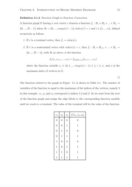
Chapter 3. Introduction to Binary Decision Diagrams 15Definition 3.1.2 Function Graph to Function ConnectionA function graph G having a root vertex v denotes a function f v : R 1 × R 2 × ... × R n →{0, ..., M − 1} where R i = {0, ..., range(v ′ ) − 1}, index(v ′ ) = i and i ∈ {1, ..., n}, definedrecursively as follows.1. If v is a terminal vertex, then f v = value(v).2. If v is a nonterminal vertex with index(v) = i, then f v : R i × R i+1 × ... × R n →{0, ..., M − 1}, with R i as above, is the functionf v (x i , x i+1 , ..., x n ) = f child(v,xi )(x i+1 , ..., x n )where the function variable x i ∈ (0, 1, ..., range(v) − 1), 1 ≤ i ≤ n, and n is themaximum index of vertices in G.□The function related to the graph in Figure 3.1 is shown in Table 3.1. The number ofvariables of the function is equal to the maximum of the indices of the vertices, namely 3in this example. x 1 , x 2 and x 3 correspond to indices 1,2 and 3. So we start from the rootof the function graph and assign the edge labels to the corresponding function variableuntil we reach to a terminal. The value of the terminal will be the value of the function.x 1 x 2 x 3 f(x 1 , x 2 , x 3 )0 0 0 00 0 1 10 1 0 00 1 1 11 0 0 01 0 1 11 1 0 11 1 1 1