Toroidal configuration of the orbit of the electron of the hydrogen ...

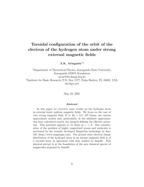
Toroidal configuration of the orbit of theelectron of the hydrogen atom under strongexternal magnetic fieldsA.K. Aringazin 1,21 Department of Theoretical Physics, Karaganda State University,Karaganda 470074 Kazakstanascar@ibr.kargu.krg.kz2 Institute for Basic Research, P.O. Box 1577, Palm Harbor, FL 34682, USAibr@gte.netMay 10, 2001AbstractIn this paper we overview some results on the hydrogen atomin external static uniform magnetic fields. We focus on the case ofvery strong magnetic field, B ≫ B 0 = 2.3 · 10 9 Gauss, use variousapproximate models and, particularly, in the adiabatic approximationhave calculated exactly the integral defining the effective potential.This potential appears to be finite at z = 0. Our considerationof the problem of highly magnetized atoms and molecules ismotivated by the recently developed MagneGas technology by Santilli(http://www.magnegas.com). The ground state electron chargedistribution of the hydrogen atom in an intense magnetic field is ofa toroidal form, in agreement with that studied by Santilli. Thisphysical picture is at the foundation of the new chemical species ofmagnecules proposed by Santilli.0

1 IntroductionWeak external static uniform magnetic field B causes anomalous Zeemansplitting of the energy levels of the hydrogen atom, with ignorably smalleffect on the charge distribution of the electron. In the case of a more intensemagnetic field which is strong enough to cause decoupling of a spin-orbitalinteraction (in atoms), e¯hB/2mc > ∆E jj ′ ≃ 10 −3 eV, i.e. B ≃ 10 5 Gauss, anormal Zeeman effect is observed, again with ignorably small deformation ofthe electron orbits.In the case of weak external magnetic field B, one can ignore the quadraticterm in the field B because its contribution is small in comparison withthat of the other terms in Schrödinger equation so that the linear approximationin the field B can be used. In such a linear approximation, the wavefunction of electron remains unperturbed, with the only effect being the wellknown Zeeman splitting of the energy levels of the hydrogen atom. In bothZeeman effects, the energy of interaction of electron with the magnetic field isassumed to be much smaller than the binding energy of the hydrogen atom,e¯hB/2mc ≪ me 4 /2¯h 2 = 13.6 eV, i.e. the intensity of the magnetic field ismuch smaller than some characteristic value, B ≪ B 0 = 2.4 · 10 9 Gauss =240000 Tesla (1 Tesla = 10 4 Gauss). Thus, the action of a weak magneticfield can be treated as a small perturbation of the hydrogen atom.In the case of very strong magnetic field, B ≫ B 0 , the quadratic term inthe field B makes a great contribution and can not be ignored. Calculationsshow that a considerable deformation of the electron charge distribution inthe hydrogen atom occurs. Namely, under the influence of a very strongexternal magnetic field a magnetic confinement takes place, i.e. in the planeperpendicular to the direction of magnetic field the electron dynamics isdetermined mainly by the action of the magnetic field, while the Coulombinteraction of the electron with the nucleus can be viewed as a small perturbation.This adiabatic approximation allows one to separate variables inSchrödinger equation [1]. At the same time, in the direction along the directionof the magnetic field the motion of electron is governed both by themagnetic field effects and the Coulomb interaction of the electron with thenucleus.In this paper we briefly review some results on the hydrogen atom in verystrong external static uniform magnetic fields, focusing on the basic physicalpicture derived from the Schrödinger equation. Our consideration of the1

problem of atoms and molecules exposed to strong external magnetic fieldis related to MagneGas technology and PlasmaArcFlow hadronic molecularreactors recently developed by Santilli [2].The highest intensities maintained macroscopically at large distances inmodern magnet laboratories are of the order of 10 5 ...10 6 Gauss (∼ 50 Tesla),i.e. much below B 0 = 2.4·10 9 Gauss (∼ 10 5 Tesla). An extremely intense externalmagnetic field, B ≥ B S = B 0 /α 2 = 4.4·10 13 Gauss, corresponds to theinteraction energy of the order of mass of electron, mc 2 = 0.5 MeV; α = e 2 /¯hcis the fine structure constant. In this case, despite the fact that the extremelystrong magnetic field does not make vacuum unstable in respect to creationof electron-positron pairs, one should account for relativistic and quantumelectrodynamics (QED) effects, and invoke Dirac or Bethe-Salpeter equation.Such intensities are not currently available in laboratories. However, theseare of interest in astrophysics, for example in studying an atmosphere ofneutron stars and white dwarfs which is characterized by B ≃ 10 9 . . . 10 13Gauss.In this paper, we shall not consider intensities as high as Schwinger valueB S , and restrict our review by the intensities 2.4 · 10 10 ≤ B ≤ 2.4 · 10 11Gauss (10B 0 . . . 100B 0 ), at which (nonrelativistic) Schrödinger equation canbe used to a very good accuracy, and the adiabatic approximation can bemade.Relativistic and QED effects (loop contributions), as well as the effectssuch as those related to the finite mass, size, and magnetic moment of thenucleus, and the finite electromagnetic radius of electron, reveal themselveseven at low magnetic field intensities, and can be accounted for as very smallperturbations. These are beyond the scope of the present paper, while beingof much importance in the high precision studies, such as those on stringenttests of the Lamb shift.It should be noted that a locally high-intensity magnetic field may arisein the plasma as the result of nonlinear effects, which can lead to creationof stable self-confined structures having a nontrivial topology with knots [3].Particularly, Faddeev and Niemi [3] recently argued that the static equilibriumconfigurations within the plasma are topologically stable solitons, thatdescribe knotted and linked fluxtubes of helical magnetic fields. In the regionclose to such fluxtubes, we suppose the magnetic field intensity may be ashigh as B 0 . In view of this, study of the action of strong magnetic field andthe fluxtubes of magnetic fields on atoms and molecules becomes of much2

interest in theoretical and applicational plasmachemistry.Possible applications are in MagneGas technology, theoretical foundationsand exciting implications of which are developed by Santilli [2]. Werefer the reader to Ref. [2] for the recent studies, description, and applicationsof MagneGas technology and PlasmaArcFlow reactors. Remarkable experimentalresults, including Gas-Chromatographic Mass-Spectroscopic andInfraRed spectrum data of Santilli’s magnegas, clearly indicates the presenceof unconventional chemical species of magnecules, which have not been identifiedas conventional molecules, and are supposed to be due to the specificbonding of a magnetic origin. The basic physical picture of the magneculesproposed by Santilli [2] is related to the toroidal orbitals of the electrons ofatoms exposed to a very strong magnetic field. The results of the presentpaper demonstrate this physical picture on the basis of the Schrödinger equation.As the result of the action of very strong magnetic field, atoms attaingreat binding energy as compared to the case of zero magnetic field. Evenat intermediate B ≃ B 0 , the binding energy of atoms greatly deviates fromthat of zero-field case, and even lower field intensities may essentially affectchemical properties of molecules of heavy atoms. This enables creation ofvarious other bound states in molecules, clusters and bulk matter [1, 2, 4].The paper by Lai [4], who focused on very strong magnetic fields, B ≫ B 0 ,motivated by the astrophysical applications, gives a good survey of the earlyand recent studies in this field, including those on the intermediate range,B ≃ B 0 , multi-electron atoms, and H 2 molecule. Much number of papersusing variational/numerical and/or analytical approaches to the problem oflight and heavy atoms, ions, and H 2 molecule in strong magnetic field, havebeen published within the last six years (see, e.g., references in [4]). However,highly magnetized molecules of heavy atoms have not been systematicallyinvestigated. One of the surprising implications is that for some diatomicmolecules of heavy atoms, the molecular binding energy is predicted to beseveral times bigger than the ground state energy of individual atoms. [5]2 Landau levels of a single electronTo estimate intensity of the magnetic field which causes a considerable deformationof the ground state electron orbit of the hydrogen atom, one can3

formally compare the Bohr radius of the hydrogen atom in the ground state,in zero external magnetic field, a 0 = ¯h 2 /me 2 ≃ 0.53 · 10 −8 cm = 1 a.u., withthe radius of orbit of a single electron moving in the external static uniformmagnetic field ⃗ B. Below, we give a brief summary of the latter issue.x-1 1 -0.5 0 y00.5 -0.50.51-14z20Figure 1: Classical orbit of the electron in an external static uniform magneticfield B ⃗ = (0, 0, B) pointed along the z axis. The electron experiences acircular motion in the x, y plane and a linear motion in the z direction (ahelical curve).The mean radius of the orbital of a single electron moving in a staticuniform magnetic field can be calculated exactly using Schrödinger equation,and is given by√n + 1/2R n = , (2.1)γwhere we have denotedγ = eH2¯hc , (2.2)B is the intensity of the magnetic field pointed along the z axis, ⃗ B = (0, 0, B),⃗r = (r, ϕ, z) in cylindrical coordinates, and n = 0, 1, . . . is the principalquantum number. Thus, the radius of the orbit takes discrete set of values(2.1), and is referred to as Landau radius. This is in contrast to the wellknown classical motion of electron in the external magnetic field (a helical4

curve is shown in Fig. 1), with the radius of the orbit being of a continuousset of values. The classical approach evidently can not be applied to studydynamics of the electron at atomic distances.Corresponding energy levels E n of a single electron moving in the externalmagnetic field are referred to as Landau energy levels,whereE n = E ⊥ n + E ‖ k z= ¯hΩ(n + 1 2 ) + ¯h2 k 2 z2m , (2.3)Ω = eH (2.4)mcis so called cyclotron frequency, and ¯hk z is a projection of the electron’smomentum ¯h ⃗ k on the direction of the magnetic field, −∞ < k z < ∞, m isthe mass of electron, and −e is the charge of electron.Landau energy levels En⊥ correspond to a discrete set of round orbitsof electron which are projected to the transverse plane. The energy E ‖ k zcorresponds to the free motion of electron in parallel to the magnetic field(continuous spectrum), with a conserved momentum ¯hk z along the magneticfield.Regarding the above presented review of Landau’s results, we remindthat in the general case of uniform external magnetic field the coordinateand spin components of the total wave function of the electron can alwaysbe separated.The corresponding coordinate component of the total wave function ofthe electron, obtained as an exact solution of Schrödinger equation for asingle electron moving in the external magnetic field with vector-potentialchosen as A r = A z = 0, A ϕ = rH/2),−(∂ ¯h2r 2 + 1 2m r ∂ r + 1 )r 2 ∂2 ϕ + ∂z 2 − γ 2 r 2 + 2iγ∂ ϕ ψ = Eψ, (2.5)is of the following form [1]:ψ n,s,kz (r, ϕ, z) =where I ns (ρ) is Laguerre function,√2γI ns (γr 2 ) eilϕ√2πe ikzz√L, (2.6)I ns (ρ) = 1 √n!s!e −ρ/2 ρ (n−s)/2 Q n−ss (ρ); (2.7)5

Q n−ss is Laguerre polynomial, L is normalization constant, l = 0, ±1, ±2, . . .is azimuthal quantum number, s = n − l is the radial quantum number, andwe have denoted, for brevity,ρ = γr 2 . (2.8)The wave function (2.6) depends on the angle ϕ as exp[ilϕ], and the energy(2.3) does not depend on the azimuthal quantum number l, so the systemreveals a rotational symmetry in respect to the angle ϕ and all the Landauorbits are round.Also, the energy (2.3) does not depend on the radial quantum numbers. This means a degeneracy of the system in respect to the position of thecenter of the orbit, and corresponds to an ”unfixed” position of the center.At n − s > 0, the origin of the coordinate system is inside the orbit while atn − s < 0 it is outside the orbit. The mean distance d between the origin ofcoordinate system and the center of orbit takes a discrete set of values, andis related to the quantum number s as follows:√s + 1/2d = . (2.9)γClearly, the energy (2.3) does not depend on this distance because of thehomogeneity of the magnetic field, so it does not depend on s. However,it should be noted that the whole Landau orbit can not move on the (r, ϕ)plane continuously along the variation of the coordinate r. Instead, it canonly ”jump” to a certain distance, which depends on the intensity of themagnetic field, in accord to Eq. (2.9).The spin components of the total wave function are triviallyψ( 1 2 ) = (10with the corresponding energiesto be added to the energy (2.3). Here,), ψ(− 1 2 ) = (01), (2.10)E spin = ±µ 0 B, (2.11)µ 0 = e¯h2mc ≃ 9.3 · 10−21 erg · Gauss −1 = 5.8 · 10 −9 eV · Gauss −1 (2.12)6

is Bohr magneton. Below, we do not consider the energy (2.11) related to theinteraction of the spin of electron with the external magnetic field becauseit decouples from the orbital motion and can be accounted for separately.As to the numerical estimation, at B = B 0 = 2.4 · 10 9 Gauss, the energyE spin ≃ ±13.6 eV.For the ground level, i.e. at n = 0 and s = 0, and zero momentum of theelectron in the z-direction, i.e. ¯hk z = 0, we have from (2.3)E ⊥ 0= e¯hB2mc , (2.13)and due to Eq. (2.6) the corresponding normalized ground state wave functionisψ 000 (r, ϕ, z) = ψ 000 (r) =√ γπ e−γr2 /2 , (2.14)∫ ∞0∫ 2π0 rdrdϕ |ψ 000 | 2 = 1.0.50.4psi0.30.20.100 1 2 3 4 5 6r, a.u.Figure 2: Landau ground state wave function of a single electron, ψ 000 (solidcurve), Eq. (2.14), in strong external magnetic field B = B 0 = 2.4 · 10 9Gauss, as a function of the distance r in cylindrical coordinates, and (fora comparison) the hydrogen ground state wave function (at zero externalmagnetic field), (1/ √ π)e −r/a 0(dashed curve), as a function of the distancer in spherical coordinates. The associated probability densities are shown inFig. 3; 1 a.u. = a 0 = 0.53 · 10 −8 cm.7

0.60.50.4Landau0.30.20.100 1 2 3 4 5 6r, a.u.Figure 3: The probability density for the case of the Landau ground stateof a single electron, 2πr|ψ 000 | 2 (solid curve), Eq. (2.14), in the strong externalmagnetic field B = B 0 = 2.4 · 10 9 Gauss, as a function of the distancer in cylindrical coordinates, and (for a comparison) probability densityof the hydrogen atom ground state (at zero external magnetic field),4πr 2 |(1/ √ π)e −r/a 0| 2 (dashed curve), as a function of the distance r in sphericalcoordinates. The associated wave functions are shown in Fig. 2; 1 a.u.= 0.53 · 10 −8 cm.The corresponding (smallest) Landau radius of the orbit of electron isin terms of which ψ 000 readsR 0 =√¯hceB ≡ √12γ , (2.15)ψ 000 =√12πR 2 0e − r24R 2 0 . (2.16)Figure 2 depicts ground state wave function of a single electron, ψ 000 ,in strong external magnetic field B = B 0 = 2.4 · 10 9 Gauss (R 0 = 1 a.u.),and (for a comparison) of the hydrogen ground state wave function, at zeroexternal magnetic field, (1/ √ π)e −r/a 0. Figures 3 and 4 display the associatedprobability density of electron as a function of the distance r from the centerof the orbit, the radius of which is about 1 a.u.8

210-1-2-2 -1 0 1 2Figure 4: A contour plot of the (r, ϕ) probability density for the case ofthe Landau ground state of a single electron, 2πr|ψ 000 | 2 , Eq. (2.14), in thestrong external magnetic field B = B 0 = 2.4 · 10 9 Gauss, as a function of thedistance in a.u. (1 a.u. = 0.53 · 10 −8 cm). Lighter area corresponds to higherprobability to find electron. The set of maximal values of the probabilitydensity is referred to as an ”orbit”.The condition that the Landau radius R 0 is smaller than the Bohr radius,R 0 < a 0 , which is adopted here as the condition of a considerable ”deformation”of the electron orbit of the hydrogen atom, then impliesB > B 0 = m2 ce 3¯h 3 = 2.351 · 10 9 Gauss, (2.17)where m is mass of electron. Equivalently, this deformation condition correspondsto the case when the binding energy of the hydrogen atom, |E0 Bohr | =|−me 4 /2¯h 2 | = 0.5 a.u. = 13.6 eV, is smaller than the ground Landau energyE0 ⊥ .The above critical value of the magnetic field, B 0 , is naturally taken asan atomic unit for the strength of the magnetic field, and corresponds to the9

case when the pure Coulomb interaction energy of electron with nucleus isequal to the interaction energy of a single electron with the external magneticfield, |E0 Bohr | = E0 ⊥ = 13.6 eV, or equivalently, when the Bohr radius is equalto the Landau radius, a 0 = R 0 = 0.53 · 10 −8 cm.It should be stressed here that we take the characteristic parameters,Bohr energy |E0 Bohr | and Bohr radius a 0 , of the hydrogen atom with a singlepurpose to establish criterium for the critical strength of the external magneticfield, for the hydrogen atom under consideration. For other atoms thecritical value of the magnetic field may be evidently different.3 Hydrogen atom in magnetic fieldsAfter we have considered quantum dynamics of a single electron in the externalmagnetic field, we turn to consideration of the hydrogen atom in theexternal static uniform magnetic field.We choose cylindrical coordinate system (r, ϕ, z), in which the externalmagnetic field is ⃗ B = (0, 0, B), i.e., the magnetic field is directed along thez-axis. General Schrödinger equation for the electron moving around a fixedproton (Born-Oppenheimer approximation) in the presence of the externalmagnetic field is(− ¯h2 ∂r 2 + 1 2m r ∂ r + 1 r 2 ∂2 ϕ + ∂z 2 +2me 2)¯h 2√ r 2 + z − 2 γ2 r 2 + 2iγ∂ ϕ ψ = Eψ,(3.1)where γ = eH/2¯hc. Note the presence of the term 2iγ∂ ϕ , which is linear inB, and of the term −γ 2 r 2 , which is quadratic in B. The other terms do notdepend on the magnetic field B.The main problem in the nonrelativistic study of the hydrogen atom inthe external magnetic field is to solve the above Schrödinger equation andfind the energy spectrum.In this equation, we can not directly separate all the variables, r, ϕ, andz, because of the presence of the Coulomb potential, e 2 / √ r 2 + z 2 , which doesnot allow us to make a direct separation in variables r and z.Also, for the general case of an arbitrary intensity of the magnetic field,we can not ignore the term γ 2 r 2 in Eq. (3.1), which is quadratic in B, sincethis term is not small at high intensities of the magnetic field.10

For example, at small intensities, B ≃ 2.4 · 10 4 Gauss = 2.4 Tesla, theparameter γ = eH/2¯hc ≃ 1.7·10 11 cm −2 so that for 〈r〉 ≃ 0.5·10 −8 cm we getthe estimation γ 2 〈r 2 〉 ≃ 10 6 cm −2 and Landau energy ¯hΩ/2 is of the orderof 10 −4 eV, while at high intensities, B ≃ B 0 = 2.4 · 10 9 Gauss = 2.4 · 10 5Tesla, the parameter γ = γ 0 ≃ 1.7 · 10 16 cm −2 so that the estimations are:γ 2 〈r 2 〉 ≃ 10 16 cm −2 (greater by ten orders) and the ground Landau energy isabout 13.6 eV (greater by five orders).Below, we turn to approximate ground state solution of Eq. (3.1) for thecase of very strong magnetic field.3.1 Very strong magnetic fieldLet us consider the approximation of a very strong magnetic field,B ≫ B 0 = 2.4 · 10 9 Gauss. (3.2)Under the above condition, in the transverse plane the Coulomb interactionof the electron with the nucleus is not important in comparison with theinteraction of the electron with the external magnetic field. So, in accord tothe exact solution (2.6) for a single electron, one can seek for an approximateground state solution of Eq. (3.1) in the form (see, e.g. [1]) of factorizedtransverse and longitudinal parts,ψ = e −γr2 /2 χ(z), (3.3)where we have used Landau wave function (2.14), s = 0, l = 0, and χ(z)denotes the longitudinal wave function to be found. This is so called adiabaticapproximation. The charge distribution of the electron in the (r, ϕ) planeis thus characterized by the Landau wave function ∼ e −γr2 /2 , i.e. by theazimuthal symmetry.In general, the adiabatic approximation corresponds to the case when thetransverse motion of electron is totally determined by the intense magneticfield, which makes it ”dance” at its cyclotron frequency. Specifically, theradius of the orbit is then much smaller than the Bohr radius, R 0 ≪ a 0 , or,equivalently, the Landau energy of electron is much bigger than the Bohrenergy E0⊥ ≫ |E0 Bohr | = 13.6 eV. In other words, this approximation meansthat the interaction of electron with the nucleus in the transverse plane isignorably small (it is estimated to make about 2% correction at B ≃ 10 1211

Gauss), and the energy spectrum in this plane is defined solely by the Landaulevels. The remaining problem is thus to find the longitudinal energyspectrum, in the z direction.Inserting wave function (3.3) into the Schrödinger equation (3.1), multiplyingit by ψ ∗ , and integrating over variables r and ϕ in cylindrical coordinatesystem, we get the following equation characterizing the z dependenceof the wave function:(− ¯h2 d 2)2m dz + ¯h2 γ2 m + C(z) χ(z) = Eχ(z), (3.4)whereC(z) = − √ ∫ ∞γ e 2 √ dρ = −e2√ πγ e γz2 erfc( √ γ|z|), (3.5)ρ + γz2erfc(x) = 1−erf(x), and0e −ρerf(x) = √ 2 ∫xπ0e −t2 dt (3.6)is error function.In Fig. 5, the exact potential C(z) is plotted, at B = 2.4 · 10 11 Gauss =100B 0 , for which case the lowest point of the potential is about C(0) ≃ −337eV. In this case, in the (r, ϕ) plane, the hydrogen atom is characterized bythe Landau energy E0⊥ = 1360 eV ≫ 13.6 eV, Landau radius R 0 = 0.5 · 10 −9cm ≪ 0.5 · 10 −8 cm, and the cyclotron frequency is Ω = 4 · 10 18 sec −1 . For acomparison, the Coulomb potential −e 2 /|z| is also shown. One can see thatthe Coulomb potential does not reproduce the effective potential C(z) to agood accuracy at small z.The arising effective potential C(z) is of a nontrivial form, which doesnot allow us to solve Eq. (3.4) analytically. Below we approximate it bysimple potentials, to make estimation on the ground state energy and wavefunction of the hydrogen atom.3.1.1 The Coulomb potential approximationAt high intensity of the magnetic field, γ ≫ 1 so that under the conditionγ〈z 2 〉 ≫ 1 we can ignore ρ in the square root in the integrand in Eq. (3.5).12

0-50-100C, eV-150-200-250-30002·10 -9 4·10 -9 6·10 -9 8·10 -9 1·10 -8z, cm0-500Coloumb, eV-1000-1500-2000-2500-300002·10 -9 4·10 -9 6·10 -9 8·10 -9 1·10 -8z, cmFigure 5: The exact effective potential C(z) (top panel), at B = 2.4 · 10 11Gauss = 100B 0 , C(0) = −337 eV, and (for a comparison) Coulomb potential−e 2 /|z| (bottom panel).Then, one can perform the simplified integral and obtain the resultC(z) ≃ V (z) = − e2|z| , at γ〈z2 〉 ≫ 1, (3.7)which appears to be a pure Coulomb interaction of electron with the nucleus,in the z direction. Therefore, Eq. (3.4) reduces to one-dimensionalSchrödinger equation for Coulomb potential,( ¯h2d 2)2m dz + e22 |z| + ¯h2 γm + E χ(z) = 0. (3.8)13

In atomic units (e = ¯h = m = 1), using the notationE ′ = ¯h2 γm + E, n2 = 1−2E ′ , (3.9)and introducing new variablex = 2z n , (3.10)we rewrite the above equation in the following form:[ d(−dx + 1 2 4 + n ) ] χ(x) = 0, (3.11)xwhere we assume, to simplify representation, x > 0. Introducing new functionv(x),χ(x) = xe −x/2 v(x), (3.12)we get the final form of the equation,xv ′′ + (2 − x)v ′ − (1 − n)v = 0. (3.13)Note that this equation is identical to that obtained for the radial part of thethree-dimensional Schrödinger equation for the hydrogen atom, at orbitalquantum number zero. We note that it is a particular case of Cummer’sequation,xv ′′ + (b − x)v ′ − av = 0, (3.14)the general solution of which is given bywhereand1F 1 (a, b, x) =v(x) = C 1 1 F 1 (a, b, x) + C 2 U(a, b, x) (3.15)∫Γ(b) 1e xt t a−1 (1 − t) b−a−1 dt (3.16)Γ(b − a)Γ(a) 0U(a, b, x) = 1 ∫ ∞e −xt t a−1 (1 + t) b−a−1 dt (3.17)Γ(a) 0are the confluent hypergeometric functions, and C 1,2 are constants. In ourcase, a = 1 − n and b = 2.14

For the wave function χ(x), we then haveχ(x) = |x|e −|x|/2 [ C ± 1 1F 1 (1 − n, 2, |x|) + C ± 2 U(1 − n, 2, |x|) ] , (3.18)where x given by Eq. (3.10) is now allowed to have any real value, and the ”±”sign in C 1,2 ± corresponds to the positive and negative values of x, respectively(the modulus sign is used for brevity).Now we turn to the normalization issue.The first hypergeometric function 1 F 1 (1 − n, 2, x) is finite at x = 0 forany n. At big x, it diverges exponentially, unless n is an integer number,n = 1, 2, . . . , at which case it diverges polynomially.The second hypergeometric function U(1 − n, 2, x) behaves differently,somewhat as a mirror image of the first one. In the limit x → 0, it isfinite for integer n = 1, 2, 3, . . ., and diverges as 1/x for noninteger n > 1and for 0 ≤ n < 1. In the limit x → ∞, it diverges polynomially forinteger n, tends to zero for noninteger n > 1 and for n = 0, and diverges fornoninteger 0 < n < 1. In Figs. 18 and 19 of Appendix, the hypergeometricfunctions 1 F 1 (1 − n, 2, x) and U(1 − n, 2, x) for n = 0, 1/4, 1/2, 1, 3/2, 2, 5/2, 3are depicted (n may be taken, for example, n = 0.133 as well).In general, because of the prefactor xe −x/2 in the solution (3.18) whichcancels some of the divergencies arising from the hypergeometric functions,we should take into account both of the two linearly independent solutions,to get the most general form of normalizable wave functions.As a consequence, the eigenvalues may differ from those correspondingto n = 1, 2, . . . (which is an analogue of the principal quantum number inthe ordinary hydrogen atom) so that n is allowed to take some non-integervalues from 0 to ∞, provided that the wave function is normalizable.We are interested in the ground state solution, which is an even state.For even states, in accord to the symmetry of the wave function under theinversion z → −z, we haveC + 1 = C − 1 , C + 2 = C − 2 , χ ′ (0) = 0. (3.19)Also, since n = 1 gives E ′ = −1/(2n 2 ) = −1/2 a.u., we should seek anormalizable wave function for n in the interval 0 < n < 1, in order toachieve the energy value, which is lower than −1/2 a.u. If it is successful,the value n = 1 indeed does not characterize the ground state. Instead, itmay correspond to some excited state.15

One can see that the problem is in a remarkable difference from the ordinarythree-dimensional problem of the hydrogen atom, for which the principalquantum number n must be integer to get normalizable wave functions, andthe value n = 1 corresponds to the lowest energy. The distinction is due tothe fact that the additional factor x in the solution (3.18) does not cancel inthe total wave function 1 .We restrict consideration by the even state so we can focus on the x ≥ 0domain, and drop the modulus sign,χ(x) = xe −x/2 [ C ± 1 1F 1 (1 − n, 2, x) + C ± 2 U(1 − n, 2, x) ] . (3.20)In summary, the problem is to identify a minimal value of n in the interval0 < n ≤ 1, at which the wave function χ(x) represented by a combination ofthe two linearly independent solutions is normalizable and obeys the conditions(3.19).The condition χ ′ (0) = 0 implies12 e−x/2 [C 1 ((2 − x) 1 F 1 (1 − n, 2, x) + (1 − n)x 1 F 1 (2 − n, 3, x)) ++C 2 ((2 − x)U(1 − n, 2, x) − 2(1 − n)xU(2 − n, 3, x))] |x=0= 0.(3.21)The function 1 F 1 (1 − n, 2, x) is well-defined at x = 0 for any n. The functionU(1 − n, 2, x) for small x behaves as x −1 Γ −1 (1 − n) so for x = 0 it appearsto be infinite, unless n = 1. The function U(2 − n, 3, x) for small x behavesas x −2 Γ −1 (2 − n) so for x = 0 it diverges (Γ(a) is Euler gamma function).Therefore, there is no way to satisfy the above condition unless we put C 2 =0, i.e. eliminate the second hypergeometric function, U(1 − n, 2, x), as anunphysical solution. As the result, only the first hypergeometric functiondetermines the wave function, at which case it is well-defined only for integern.For the first hypergeometric function as the remaining solution, the situationis well known,1F 1 (a, b, |x|) |x=0 = 1,ddx 1 F 1 (a, b, x) |x=0 = a b . (3.22)1 In the three-dimensional Coulomb problem it does cancel in the total wave function.16

We take n = 1 as this value implies the lowest energy E ′ in this case. Theenergy for n = 1 is E ′ = −1/2 a.u., i.e.E = − me4 12− (3.23)2¯h 2¯hΩ,where we have used ¯h 2 1γ/m = 2¯hΩ due to Eqs. (2.2) and (2.4).Thus, the particular state n = 1 of the hydrogen atom is characterized byusual Bohr distance a 0 in the z direction, with the longitudinal wave functionχ(z) ≃ |z|e −|z|/a 0. (3.24)In addition, it is easy to check directly, without using the general hypergeometricfunction technique, that χ(z) = ze −z satisfies the equation ( 1 2 d2 /dz 2 +1/z + ɛ)χ(z) = 0, for ɛ = −1/2.In the (r, ϕ) plane (n = 0, s = 0) the orbit is characterized by the Landauradius R 0 ≪ a 0 , with the Landau wave function ≃ e −r2 /4R0 2 , and the Landauenergy E0⊥ given by the second term in Eq. (3.23). Thus, the n = 1 wavefunction in the Coulomb approximation is written asψ(r, ϕ, z) ≃√ γπ ze−γr2 /2−|z|/a 0=√12πR 2 0ze − r24R02 − |z|a 0. (3.25)Also, spin of the electron for the ground state is aligned antiparallel to themagnetic field.The associated probability density is evidently of a cylindrical (axial)symmetry and can be described as two Landau orbits of radius R 0 in different(r, ϕ) planes, one at the level z = −a 0 , and the other at the level z = +a 0 ,with the nucleus at z = 0, as schematically depicted in Fig. 6. Presence oftwo Landau orbits occurs in accord to the wave function (3.25), which equalszero at z = 0 and is symmetrical with respect to the inversion, z → −z. Theelectron moves simultaneously on these two orbits.The above electron charge distribution supports the study made by Santilli[2] who proposed the polarized toroidal electron orbit in the hydrogenatom under the action of strong magnetic field, but the Coulomb approximationsuggests the electron charge distribution in the form of two identicalcoaxial round orbits separated by relatively big vertical distance; see Fig. 6.Note that the size of the hydrogen atom in the z direction is predictedto be about 10 times bigger than that in the transverse plane, i.e. R 0 =17

yxzFigure 6: Schematic view on the hydrogen atom in the ground state, at verystrong external magnetic field ⃗ B = (0, 0, B), B ≫ B 0 = 2.4 · 10 9 Gauss, dueto the Coulomb approximation approach, Eq. (3.25). One electron movessimultaneously on two Landau orbits of radius R 0 which are shown schematicallyas torii in the different (x, y) planes, one torus at the level z = −a 0and the other at the level z = +a 0 , with the nucleus shown in the center atz = 0. Each torus represents the (x, y) probability distribution as shown inFig. 4 but with small Landau radius, R 0 ≪ a 0 . The spin of the electron isaligned antiparallel to the magnetic field.0.53 · 10 −9 cm ≃ 0.1a 0 ; the hydrogen atom is thus highly elongated in the zdirection (this ratio is not kept in Fig. 6). The cyclotron frequency (2.4) isof about 4 · 10 18 sec −1 . Classically, the linear velocity of the electron on suchan orbit is v = 2πR 0 Ω and is estimated to be v = 1.3 · 10 10 cm/sec ≃ 0.4c.We should to note here that Landau radius R 0 , at B = 2.4 · 10 11 Gauss= 100B 0 , is about ten times bigger than Compton wavelength of electron,λ e /2π ≃ 0.4·10 −10 cm, hence we can ignore quantum electrodynamics effects.Finally, it should be noted that the above used Coulomb approximationis rather a crude one (see Fig. 5). Indeed, the energy in the z-direction doesnot depend on the magnetic field intensity while it is obvious that it should18

depend on it. In the next Section, we approximate the effective potentialC(z) with a better accuracy.3.1.2 The modified Coulomb potential approximationWe note that due to the exact result (3.5), the effective potential C(z) tendsto zero as z → ∞ (not a surprise). However, a remarkable implication of theexact result is that C(z) is finite at z = 0, namely,C(0) = − √ πγ e 2 , (3.26)so that the effective potential C(z) indeed can not be well approximatedby the Coulomb potential, −e 2 /|z|, at small z (|z| < 10 −8 cm) despite thefact that at big values of γ (γ ≫ γ 0 ≃ 1.7 · 10 16 cm −2 ) the Coulomb potentialreproduces C(z) to a good accuracy at long and medium distances.Thus, the approximation considered in Sect. 3.1.1 appears to be not valid at(important) short distances.Consequently, Eq. (3.4) with the exactly calculated C(z) will yield theground state of electron in the z direction which is drastically different fromthat with the Coulomb potential considered in Sect. 3.1.1. Thus, very intensemagnetic field essentially affects dynamics of electron not only in the (r, ϕ)plane but also in the z direction. We expect that for the case of exactpotential (3.5) the ground state is characterized by much lower energy in thez direction as compared to that of the one-dimensional Bohr state (3.23).The exact potential C(z) can be well approximated by the modifiedCoulomb potential,e2C(z) ≃ V (z) = − , (3.27)|z| + z 0where z 0 is a parameter, z 0 ≠ 0, which depends on the field intensity B duetoz 0 = − e2C(0) = √ 1√2¯hc= πγ πeB . (3.28)The analytic advantage of this approximation is that V (z) is finite at z = 0,being of Coulomb-type form.Calculations for this approximate potential can be made in an essentiallythe same way as in the preceding Section, with |x| being replaced by |x|+x 0 ,19

where x 0 > 0 (we remind that x = 2z/n),χ(x) = (|x|+x 0 )e −(|x|+x 0)/2 [ C ± 1 1F 1 (1−n, 2, |x|+x 0 ) + C ± 2 U(1−n, 2, |x|+x 0 ) ] .(3.29)An essential difference from the pure Coulomb potential case is that thepotential (3.27) has no singularities. The x → 0 asymptotic of the associatedsecond hypergeometric function, U(1−n, 2, |x|+x 0 ) becomes well-defined fornoninteger n. Thus, the condition χ ′ (x) |x=0 = 0 does not lead to divergenciesin the second solution for noninteger n < 1. It remains only to provide welldefinedbehavior of the wave function at x → ∞.Analysis shows that normalizable wave functions, as a combination of twolinearly independent solutions, for the modified Coulomb potential does existfor various non-integer 2 n. We are interested in the ground state solution,so we consider the values of n from 0 to 1. Remind that E ′ = −1/(2n) 2 sothat for n < 1 we obtain the energy lower than −0.5 a.u.For n < 1, the first hypergeometric function is not suppressed by theprefactor xe −x/2 in the solution (3.29) at large x so we are led to discard it asan unphysical solution by putting C 1 = 0. A normalizable ground state wavefunction for n < 1 is thus may be given by the second term in the solution(3.29). The condition χ ′ (x) |x=0 = 0 implies12 e−(x+x 0)/2 C 2 [(2 − x − x 0 )U(1 − n, 2, x + x 0 )−−2(1 − n)(x + x 0 )U(2 − n, 3, x + x 0 ))] |x=0 = 0.(3.30)The l.h.s of this equation depends on n and x 0 , so we can select some fieldintensity B, calculate associated value of the parameter x 0 = x 0 (B) and findthe value of n, from which we obtain the ground state energy E ′ .On the other hand, for the ground state this condition can be viewed,vice versa, as an equation to find x 0 for some given value of n [6]. Hereby wereverse the order of the derivation, to simplify numerical calculations.For example, taking the noninteger valuewe find from Eq. (3.30) numericallyn = 1/ √ 15.58 ≃ 0.253 < 1 (3.31)x 0 = 0.140841. (3.32)2 This is the case when one obtains a kind of ”fractional” quantum number n whichdoes make sense.20

This value is in confirmation with the result x 0 = 0.141 obtained by Heyl andHernquist [6] (see Discussion). On the other hand, x 0 is related in accord toEq. (3.28) to the intensity of the magnetic field,x 0 = 2z 0n = √8¯hcπn 2 eB , (3.33)from which we obtain B ≃ 4.7 · 10 12 Gauss. Hence, at this field intensitythe ground state energy of the hydrogen atom is given by E ′ = −1/(2n 2 ) =−15.58 Rydberg.0.80.6n=0.253, x0=0.141chi0.40.20-10 -5 0 5 10xFigure 7: The longitudinal ground state wave function χ(x), Eq. (3.34), ofthe hydrogen atom in the magnetic field B = 4.7 · 10 12 Gauss; n = 1/ √ −2E,x = 2z/n.The longitudinal ground state wave function is given byχ(x) ≃ (|x| + x 0 )e (|x|+x 0)/n U(1 − n, 2, |x| + x 0 ), (3.34)and is plotted in Fig. 7). The total wave function is√1χ(x) ≃ e − r24R 22πR02 0 (|x| + x 0 )e (|x|+x0)/n U(1 − n, 2, |x| + x 0 ), (3.35)and the associated three-dimensional probability density is schematically depictedin Fig. 8.In contrast to the double Landau-type orbit implied by the Coulombpotential approximation, the modified Coulomb potential approach provides21

zyxFigure 8: Schematic view of the hydrogen atom in the ground state, at verystrong external magnetic field B ⃗ = (0, 0, B), B ≫ B 0 = 2.4 · 10 9 Gauss,due to the modified Coulomb approximation approach. The electron moveson the Landau orbit of small radius R 0 ≪ 0.53 · 10 −8 cm, which is shownschematically as a torus. The vertical size of the atom is comparable to R 0 .Spin of the electron is aligned antiparallel to the magnetic field.qualitatively correct behavior and much better accuracy, and suggests a singleLandau-type orbit shown in Fig. 8 for the ground state charge distributionof the hydrogen atom. This is in full agreement with Santilli’s study [2] ofthe hydrogen atom in strong magnetic field.Only excited states are characterized by the double Landau-type orbitsdepicted in Fig. 6. We shall not present calculations for the excited states inthe present paper, and refer the reader to Discussion for some details on theresults of the study made by Heyl and Hernquist [6].3.1.3 Variational and numerical solutionsReview of approximate, variational, and numerical solutions can be foundin the paper by Lai [4]. Accuracy of numerical solutions is about 3%, forthe external magnetic field in the range from 10 11 to 10 15 Gauss. Figure 9reproduces Fig. 1 of Ref. [4]. It represents the computed ionization energyQ 1 of the hydrogen atom and dissociation energy of H 2 molecule as functions22

Figure 9: Ionization energies of the hydrogen atom and H 2 molecule exposedto very strong magnetic field; B 12 = B · 10 −12 Gauss (reproduction of Fig. 1by Lai [4]).of the intensity of the magnetic field; B 12 = B · 10 −12 Gauss, i.e. B 12 = 1means B = 10 12 Gauss.z size L, a.u.0.210.20.190.180.170.160.150 200 400 600 800 1000bFigure 10: Longitudinal z-size of the hydrogen atom in the magnetic field, Eq.(3.36), as a function of the magnetic field intensity; b = B/B 0 , B 0 = 2.4 · 10 9Gauss, 1 a.u. = 0.53 · 10 −8 cm.Due to the variational results [4], the z-size of the hydrogen atom in the23

Transverse size L, a.u.0.10.090.080.070.060.050.040.030 200 400 600 800 1000bFigure 11: Transverse size of the hydrogen atom in the magnetic field, Eq.(3.37), as a function of the magnetic field intensity; b = B/B 0 , B 0 = 2.4 · 10 9Gauss, 1 a.u. = 0.53 · 10 −8 cm.ground state is well approximated by the formula (Fig. 10)L z ≃1ln(B/B 0 )the transverse (Landau) size is (Fig. 11)L ⊥ ≃a.u.; (3.36)1√B/B 0a.u.; (3.37)and the ground state energy is (Fig. 12)E ≃ −0.16[ln(B/B 0 )] 2 a.u., (3.38)with the accuracy of few percents, for b ≡ B/B 0 in the range from 10 2 to10 6 .One can see for B = 100B 0 , that the variational study predicts the groundstate energy E = −3.4 a.u. = −92.5 eV (much lower than the value, −0.5a.u., predicted by the n = 1 Coulomb approximation in Sect. 3.1.1), thetransverse size L ⊥ of about 0.1 a.u. (the same as in the Coulomb approximation)and the z-size L z of about 0.22 a.u. (much smaller than the value,1 a.u., predicted by the Coulomb approximation). This confirms the resultof the approximate analytic approach, in which n < 1 implies ground stateenergy much lower than −0.5 a.u.24

Energy E, a.u.-4-5-6-70 200 400 600 800 1000bFigure 12: Variational ground state energy of the hydrogen atom in themagnetic field, Eq. (3.38), as a function of the magnetic field intensity;b = B/B 0 , B 0 = 2.4 · 10 9 Gauss, 1 a.u. = 27.2 eV.4 DiscussionIn a physical context, the used adiabatic approximation implies that theposition of the nucleus is not ”fixed” in the (r, ϕ) plane. Indeed, there is noreason for the nucleus to stay ”exactly” at the center of the orbit when theCoulomb force in the transverse plane is totally ignored.In contrast, in the z direction, we have more complicated situation,namely, the magnetic field leads to the effective interaction potential C(z),which is finite at z = 0 and is Coulomb-like in the long-range asymptotic.Hence, the position of the nucleus remains to be fixed in the z directionrelative to the orbit of the electron (bound state).Due to the (crude) Coulomb approximation of Sect. 3.1.1, the electronprobability density of the hydrogen atom under very intense magnetic field,at n = 1, appears to be of rather nontrivial form schematically depicted inFig. 6.More accurate approach may yield some different electron charge distributionsbut we expect that the symmetry requirements (namely, the axialsymmetry and the (anti)symmetry under inversion z → −z) would lead againto a toroidal orbit, which is splitted into two identical coaxial orbits (the toriiare separated) similar to that shown in Fig. 6, or to an unsplitted one (thetwo torii are superimposed) as shown in Fig. 8.Accurate analytic calculation of the ground and excited hydrogen wave25

functions made by Heyl and Hernquist [6] in the adiabatic approximationleads to the longitudinal parts of the wave functions (the vertical z dependence)shown in Fig. 13, which reproduces the original Fig. 3 of their work;ζ = 2παz/λ e ; B = 4.7 · 10 12 Gauss. They used the modified Coulomb potentialof the type (3.27), and the additional set of linearly independent solutionsof the one-dimensional modified Coulomb problem in the form∫(|x| + x m )e −(|x|+x |x|+xmm)/21 F 1 (1 − n, 2, |x| + x m )e t(t 1 F 1 (1 − n, 2, t)) 2 dt,(4.1)where m = 0 corresponds to the ground state. For the ground state with n =1/ √ 15.58, i.e. the binding energy is 15.58 Rydberg, they found x 0 = 0.141,which corresponds to B = 4.7 · 10 12 Gauss. This result is in agreement withthe study made in Sect. 3.1.2.Figure 13: The axial wavefunctions of hydrogen in an intense magnetic field(analytic calculation) for B = 4.7·10 12 Gauss. The first four even states withaxial excitations, |000〉 (ground state), |002〉, |004〉, and |006〉 (left panel), andodd states |001〉 and |003〉 (right panel) are depicted. Here, B = 4.7 · 10 12Gauss, ground state energy is E = −15.58 Rydberg, n = 1/ √ 15.58, ζ =2z/n corresponds to x in our notation; z in a.u., 1 a.u. = 0.53 · 10 −8 cm(reproduction of Figure 3 by Heyl and Hernquist [6]).26

Figure 14: The axial ground state |000〉 wavefunction of hydrogen in anintense magnetic field, analytic calculation (solid curve) and numerical result(dashed line); B = 4.7 · 10 12 Gauss, E = −15.58 Rydberg, n = 1/ √ 15.58,ζ = 2z/n corresponds to x in our notation; z in a.u., 1 a.u. = 0.53 · 10 −8 cm(reproduction of Figure 4 by Heyl and Hernquist [6]).One can see from Fig. 13 that the peak of the ground state wave function|000〉 is at the point z = 0 (see also Fig. 14 for a close view) while the largestpeaks of the excited wave functions are away from the point z = 0 (as itwas expected to be). Consequently, the associated longitudinal probabilitydistributions (square modules of the wave functions multiplied by the volumefactor of the chosen coordinate system) are symmetric with respect to z →−z, and their maxima are placed in the center z = 0 for the ground state,and away from the center for the excited states.In contrast to the double toroidal orbit (Fig. 6) implied by the Coulombapproximation of Sect. 3.1.1, the modified Coulomb potential approach suggestsa single toroidal orbit (Fig. 8) for the ground state charge distributionof the hydrogen atom. This confirms Santilli’s study [2] of the hydrogenatom in strong magnetic field. The excited states |00ν〉 are characterized bya double toroidal orbit schematically depicted in Fig. 6.The computed ground state |000〉 binding energy of the hydrogen atomfor different field intensities are [6]:27

Magnetic field B(Gauss)Binding energy, |000〉 state(Rydberg)4.7 × 10 12 15.589.4 × 10 12 18.8023.5 × 10 12 23.814.7 × 10 13 28.229.4 × 10 13 33.2123.5 × 10 13 40.754.7 × 10 14 47.20They calculated first-order perturbative corrections to the above energiesand obtained the values, which are in a good agreement with the results byLai [4] (see Fig. 9) and Ruder et al. [1].It is remarkable to note that in very strong magnetic field, the energydifferences between the excited states and the ground state of the hydrogenatom are small in comparison to the absolute value of the ground state energy.The excited states are represented by the double torii configurations sincethe peaks of the associated wave functions spread far away from the centerz = 0 in both +z and −z directions.The above ground state electron charge distributions strongly support thestudy made by Santilli [2] who proposed the polarized toroidal electron orbitin the hydrogen atom under the action of strong magnetic field as a physicalpicture at the foundation of the new chemical species of magnecules. Theonly addition to this picture is that the the excited states are characterizedby the double torii configuration.Since zero field ground state case is characterized by perfect sphericallysymmetric electron charge distribution of the hydrogen atom, intermediateintensities of the magnetic field are naturally expected to imply a distortedspherical distribution. However, deeper analysis is required for the intermediatemagnetic field intensities because the adiabatic approximation is notlonger valid in this case. Namely, an interesting problem is to solve theSchrödinger equation (3.1) for the case when intensity of the magnetic fieldis not very strong, B ≤ B 0 , with the corresponding characteristic Landauground state energy of about the Bohr energy. In this case, both the Coulomband magnetic interactions should be taken at the same footing that leads tocomplications in its analytic study.28

Figure 15: Ionization energies of He atom exposed to very strong magneticfield (numerical solutions); B 12 = B · 10 −12 Gauss (reproduction of Fig. 5 byLai [4]).As to the multi-electron atoms, an interesting problem is to study actionof a very strong external magnetic field on He atom (see. e.g., Heyl and Hernquist[6] and Lai [4]; Fig. 15) and on the multi-electron heavy atoms, withouter electrons characterized by a nonspherical charge distribution, such asthe p-electrons in Carbon atom, orbitals of which penetrate the orbitals ofinner electrons. Very intense magnetic field would force such outer electronsto follow small round Landau orbits. In addition to the effect of a directaction of the magnetic field on the inner electrons, a series of essential rearrangementsof the whole electron structure of the atom seems to be occurwith a variation of the external magnetic field strength. Indeed, the magneticfield competes with both the Coulomb energy, which is different fordifferent states of electrons, and the electron-electron interactions, includingspin pairings. However, it is evident that at sufficiently strong fields, all theelectron spins are aligned antiparallel to the magnetic field — fully spin polarizedconfiguration — while at lower field intensities various partial spinpolarized configurations are possible.29

Figure 16: Contour plots of the (r, z) plane electron density of the iron atomaccording to density matrix theory at two different magnetic field strengths,10 11 Gauss (left) and 10 12 Gauss (right). The outermost contour encloses 99%of the negative charge, the next 90%, then 80% etc., and the two innermost5% and 1% respectively (reproduction of Fig. 5 by Johnsen and Yngvason[5]).In accord to the numerical calculations based on the density matrix theoryapproach by Johnsen and Yngvason [5], which is in quite good agreementwith the result of Hartree-Fock approach at very strong magnetic field intensities,the inner domain in the iron atom (26 electrons) is characterized byslightly distorted spherically symmetric distribution even at the intensitiesas high as B = 100B 0 . . . 1000B 0 . The outer domain appears to be of specific,highly elongated distribution along the direction of the magnetic fieldas shown in Fig. 16. The possible interpretation that the inner electrons remainto have spherical distribution while outer electrons undergo the squeezeseems to be not correct unless the spin state of the iron atom is verified tobe partially polarized. So, we can conclude that all the electrons are in30

highly magnetically polarized state (Landau state mixed a little by Coulombinteraction), and the electron structure is a kind of Landau multi-electroncylindrical shell, with spins of all the electrons being aligned antiparallel tothe magnetic field (fully spin polarized configuration).Another remark regarding Fig. 16 is that the contours indicating nearlyspherical distribution will always appear since the Coulomb center (nucleus)is not totally eliminated from the consideration (non-adiabatic approximation),and it forces a spherical distribution to some degree, which evidentlydepends on the distance from the center (closer to the center, more sphericity).We note that Fig. 16 is in qualitative agreement with Fig. 6 in the sensethat the predicted charge distribution reveals symmetry under the inversionz → −z, with the characteristic z-elongated toroidal orbits.An exciting problem is to study H 2 molecule under the action of strongexternal static uniform magnetic field using Schrödinger equation. Since thebinding energy of H 2 molecule is of about 4.75 eV (much less than 13.6 eV ofindividual hydrogen atoms) and two interacting electrons of spin 1/2 participatedynamics we expect interesting physical predictions. For example, itis interesting to analyze the problem of bonding, in the presence of a strongmagnetic field.However, before studying H 2 molecule it would be very useful to investigatemuch simpler two-center system, H 2+ ion, as it can give valuable informationon the features of a two-center system under the action of a strongmagnetic field. We refer the interested reader to Refs. [4, 6] for details ofstudies on H + 2 ion and H 2 molecule in strong magnetic field. Figure 17 displaysground and first excited state wave functions of H 2+ ion calculated byHeyl and Hernquist [6].Finally, it should be noted that studies on the atomic and molecularsystems in strong magnetic fields and related issues are becoming extensivelast years. We refer the reader to a recent review by Lai [4] for an extensivelist of references, and below present summary of some selected recent papers.The work by Kravchenko et al. [8] uses an orthogonal approach andachieves very high precision by solving the general problem of the hydrogenatom in an arbitrarily strong magnetic field. This analytical work is of muchimportance as it provides solid ground to analyze few-electron and multielectronatoms, and simple diatomic molecules.A series of papers by Schmelcher et al. [9] is devoted to a systematic studyof various simple atomic, ionic and molecular systems in strong magnetic31

Figure 17: The ground and first-excited state of H + 2 ion. The solid line traces|000〉, and the dashed line follows |0 -1 0〉. The triangles give the positionsof the protons for the ground state and the squares for the excited state.Magnetic field B = 4.7 · 10 12 Gauss is pointed along the internuclear axis;ζ = 2παz/λ e denotes z in a.u.; 1 a.u. = 0.53 · 10 −8 cm (reproduction ofFigure 5 by Heyl and Hernquist [6]).fields via Hartree-Fock method. One of the papers by Schmelcher et al.considers the carbon atom.Analytical approximations have been constructed by Potekhin [10] forbinding energies, quantum mechanical sizes and oscillator strengths of mainradiative transitions of hydrogen atoms arbitrarily moving in magnetic fields≃ 10 12 . . . 10 13 Gauss. This approach is of much importance in investigatingan interaction of highly magnetized hydrogen atoms in a gaseous phase.Computational finite element method for time-dependent Schrödingerequation has been developed by Watanabe and Tsukada [11] to study dynamicsof electrons in a magnetic field that can be used effectively for mesoscopicsystems, such as small clusters.32

AcknowledgementsThe author is much grateful to R.M. Santilli for discussions and support.Additional thanks are due to M.I. Mazhitov, Karaganda State University,for stimulating discussions.33

Appendix2000201500151F11000U10500500 2 4 6 8 10x, n=000 2 4 6 8 10x, n=01F160050040030020010000 2 4 6 8 10x, n=1/4U201510500 2 4 6 8 10x, n=1/41F140030020010000 2 4 6 8 10x, n=1/2U17.51512.5107.552.500 2 4 6 8 10x, n=1/221.521.51F11U10.50.500 2 4 6 8 10x, n=100 2 4 6 8 10x, n=1Figure 18: The confluent hypergeometric functions 1 F 1 (1−n, 2, x) and U(1−n, 2, x) for various n.34

1F10-5-10-15-20-25-30-350 2 4 6 8 10x, n=3/2U2.50-2.5-5-7.5-10-12.50 2 4 6 8 10x, n=3/210861F1-1-2-3-40 2 4 6 8 10x, n=2U420-20 2 4 6 8 10x, n=21F12.521.510.50-0.50 2 4 6 8 10x, n=5/2U25201510500 2 4 6 8 10x, n=5/21F1543210U3025201510500 2 4 6 8 10x, n=30 2 4 6 8 10x, n=3Figure 19: The confluent hypergeometric functions 1 F 1 (1−n, 2, x) and U(1−n, 2, x) for various n.35

References[1] A.A. Sokolov, I.M. Ternov, V.Ch. Zhukovskii, Quantum mechanics(Moscow, Nauka, 1979) (in Russian);L.D. Landau and E.M. Lifshitz, Quantum Mechanics: Non-RelativisticTheory, 3rd ed. (Pergamon, Oxford, 1989).H. Ruder, G. Wunner, H. Herold, F. Geyer, Atoms in Strong MagneticFields (Springer, Berlin-Heidelberg-New York, 1994);B.B. Kadomtsev, Soviet Phys. JETP 31 (1970) 945; B.B. Kadomtsevand V.S. Kudryavtsev, JETP 13 (1971) 42; B.B. Kadomtsev andV.S. Kudryavtsev, JETP Lett. 13 (1971) 9.[2] R.M. Santilli, Hadronic J. 21, 789 (1998);R.M. Santilli, The Physics of New Clean Energies and Fuels Accordingto Hadronic Mechanics, Journal of New Energy 4, Special Edition, No.1 (1999), 318 pages;R.M. Santilli and D.D. Shillady, Intern. J. Hydrogen Energy 24, 943(1999); Intern. J. Hadrogen Energy 25, 173 (2000);R.M. Santilli, Hadronic Chemistry, With Applications to New Clean Energiesand Fuels (2001), to appear;http://www.magnegas.com[3] L. Faddeev and A.J. Niemi, Magnetic geometry and the confinement ofelectrically conducting plasmas, physics/0003083, April 2000.R. Battye, P. Sutcliffe, Phys. Rev. Lett. 81 (1998) 4798; and Proc. R.Soc. Lond. A455 (1999) 4305.J. Hietarinta, P. Salo, Phys. Lett. B451 (1999) 60; and The groundstate in theFaddeev-Skyrme model, University of Turku preprint, 1999; For videoanimations, see http://users.utu.fi/hietarin/knots/index.html[4] D. Lai, Matter in strong magnetic fields, chem-ph/0009333, September2000.[5] K. Johnsen and J. Yngvason, Density Matrix Functional Calculationsfor Matter in Strong Magnetic Fields: I. Atomic Properties, chemph/9603005,March 1996.36

[6] J.S. Heyl and L. Hernquist, Hydrogen and Helium Atoms and Moleculesin an Intense Magnetic Field, chem-ph/9806040, June 1998;M.D. Jones, G. Ortiz, and D.M. Ceperley, Spectrum of Neutral Heliumin Strong Magnetic Fields, chem-ph/9811041, November 1998.[7] J.C. Lopez, P. Hess, and A. Turbiner, H 2 + ion in strong magnetic field:a variational study, Preprint ICN-UNAM 97-06, chem-ph/9707050;A. Turbiner, J.C. Lopez, and U. Solis, H 3 ++ molecular ions can exist instrong magnetic fields, Preprint ICN-UNAM 98-05, chem-ph/9809298;J.C. Lopez and A. Turbiner, One-electron linear systems in a strongmagnetic field, Preprint ICN-UNAM 99-03, chem-ph/9911535.[8] Yu.P. Kravchenko, M.A. Liberman and B. Johansson, Phys. Rev. Lett.77 (1996) 619.[9] T. Detmer, P. Schmelcher and L.S. Cederbaum, Hydrogen molecule in amagnetic field: The lowest states of the Π manifold and the global groundstate of the parallel configuration, chem-ph/9711003;T. Detmer, P. Schmelcher, F.K. Diakonos and L.S. Cederbaum, The hydrogenmolecule in magnetic fields: The ground states of the Σ manifoldof the parallel configuration, chem-ph/9711020;M.V. Ivanov and P. Schmelcher, The ground state of the lithium atomin strong magnetic fields, chem-ph/9801014;D.M. Leitner and P. Schmelcher, Mesoscopic motion of atomic ions inmagnetic fields, chem-ph/9808020;W. Becken, P. Schmelcher and F.K. Diakonos, The helium atom in astrong magnetic field, chem-ph/9902059;P. Schmelcher, M.V. Ivanov, and W. Becken, Exchange and correlationenergies of ground states of atoms and molecules in strong magneticfields, chem-ph/9902060;V.S. Melezhik and P. Schmelcher, Magnetic field stimulated transitionsof excited states in fast muonic Helium ions, chem-ph/9909030;M.V. Ivanov and P. Schmelcher, The ground state of the carbon atom instrong magnetic fields, chem-ph/9909031;P. Schmelcher and L.S. Cederbaum, Magnetic field induced two-bodyphenomena in atoms, chem-ph/9909045;37

M.V. Ivanov and P. Schmelcher, Ground states of the atoms H, He,. . . ,Ne and their singly positive ions in strong magnetic fields: The high fieldregime, chem-ph/9910017;O.-A. Al-Hujaj and P. Schmelcher, Ground and excited states of thehydrogen negative ion in strong magnetic fields, chem-ph/0003043;V.G. Bezchastnov, P. Schmelcher, and L.S. Cederbaum, Bound states ofnegatively charged ions induced by a magnetic field, chem-ph/0006016;M.V. Ivanov and P. Schmelcher, Finite-difference calculations for atomsand diatomic molecules in strong magnetic and static electric fields,chem-ph/0006017;P. Schmelcher, T.Detmer and L.S. Cederbaum, Excited states of thehydrogen molecule in magnetic fields: The singlet Σ states of the parallelconfiguration, chem-ph/0006018;V.S. Melezhik and P. Schmelcher, Quantum energy flow in atomic ionsmoving in magnetic fields, chem-ph/0006019.[10] A.Y. Potekhin, Hydrogen atom moving across a strong magnetic field:analytical approximations, chem-ph/9710046.[11] N. Watanabe and M. Tsukada, Finite element approach for simulatingquantum electron dynamics in a magnetic field, Journal of PhysicalSociety of Japan 69, No. 9 (2000) 2962, chem-ph/0011069.38