Optimal Stopping and Applications

Optimal Stopping and ApplicationsAlex CoxMarch 16, 2009AbstractThese notes are intended to accompany a Graduate course on Optimal stopping,and in places are a bit brief. They follow the book ‘Optimal Stopping and FreeboundaryProblems’ by Peskir and Shiryaev, and more details can generally befound there.1 Introduction1.1 Motivating ExamplesGiven a stochastic process X t , an optimal stopping problem is to compute the following:sup EF(X τ ), (1)τwhere the supremum is taken over some set of stopping times. As well as computing thesupremum, we will also usually be interested in finding a description of the stopping time.For motivation, we consider three applications where optimal stopping problems arise.(i) Stochastic analysis. Let B t be a Brownian motion. Then classical results tell usthat for any (fixed) T ≥ 0,[ ] √πTE sup |B s | =0≤s≤T 2What can we say about the left-hand side if we replace the constant T with astopping time τ? To solve this problem, it turns out that we can consider the (classof) optimal stopping problems:V (λ) = sup Eτ[]sup |B s | − λτ0≤s≤τ. (2)Where we take the supremum over all stopping times which have Eτ < ∞, andλ > 0. (Note that in order to fit into the exact form described in (1), we need1

Optimal Stopping and Applications — Introduction Amg Cox 2to take e.g. X t = (B t , sup s≤t |B s |, t)). Now suppose we can solve this problem forall λ > 0, then we can use a Lagrangian-style approach to get back to the originalquestion: for any suitable stopping time τ we have[ ]E sup |B s | ≤ V (λ) + λEτ0≤s≤τ≤ inf (V (λ) + λEτ)λ>0Now, if we suppose that the infimum here is attained, and the supremum in (2) isalso attained at the optimal λ, then we see that the right-hand side is a functionof Eτ, and further, we can attain equality for this bound, so that it is the smallestpossible bound.(ii) Sequential analysis. Suppose we observe (in continuous time) a statistical processX t — perhaps X t is a measure of the health of patients in a clinical trial. We wishto know whether a particular drug has a positive impact on the patients. If wesuppose that the process X t has:X t = µt + B twhere µ is the unknown effect of the treatment. Then to make inference, we mighttest the hypotheses:H 0 : µ = µ 0 , H 1 : µ = µ 1 .Our goal might be to minimise the average time we take to make a decision subjectto some constraints on the probabilities of making wrong decisions:P(accept H 0 |H 1 true) ≤P(accept H 1 |H 0 true) ≤ β.Again, using Lagrangian techniques, we are able to rewrite this as an optimal stoppingproblem, which we can solve to find the optimal stopping time (together witha ‘rule’ to decide whether we accept or reject when we stop).(iii) Mathematical Finance. Let S t be the share price of a company. A common typeof option is the American Put option. This contract gives the holder of the optionthe right, but not the obligation, to sell the stock for a fixed price K to the writerof the contract at any time before some fixed horizon T. In particular, suppose theholder exercises at a stopping time τ, then the discounted 1 value of the payoff is:e −rτ (K − S τ ) + . This is the difference between the amount she receives, and theactual value of the asset, and we take the positive part, since she will only choose toexercise the option, and sell the share, if the price she would receive is larger thanthe price she would get from selling on the market. If the holder of the contractchooses the stopping time τ, the fundamental theorem of asset pricing 2 says thatthe payoff has initial valueE Q e −rτ (K − S τ ) + ,1 We convert time-t money into time-0 money by multiplying the time-t amount by the discount factore −rt , where r is the interest rate.2 If you don’t know what this is, ignore the Q that crops up, and just think of this as pricing by takingan average of the final payoff.αPlease e-mail any comments/corrections/questions to: A.M.G.Cox@bath.ac.uk.

Optimal Stopping and Applications — Introduction Amg Cox 3where Q is the risk-neutral measure since the seller would not want to sell this toocheaply (and in fact, there is a better argument based on hedging that we will seelater), and she doesn’t know what strategy the buyer will use, so she should takethe supremum over all stopping times τ ≤ T:Price = sup E Q e −rτ (K − S τ ) + .τ≤TSo pricing the American put option is equivalent to solving an optimal stoppingproblem.1.2 Simple ExampleOnce a problem of interest has been set up as an optimal stopping problem, we then needto consider the method of solution. The exact techniques vary depending on the problem,however there are two important approaches — the martingale approach, and the Markovapproach, and there are a number of common features that any optimal stopping problemis likely to exhibit.We will now consider a reasonable simple example where we will be able to explicitlyobserve many of the common features.Let X n be a simple symmetric random walk on a probability space (Ω, F, (F n ) n∈Z+ , (P x ) x∈Z ),where F n is the natural filtration of X n , and P x (X 0 = x) = 1. Let f(·) be a function onZ with f(n) = 0 if n ≥ N or n ≤ −N, for some N. Then the optimal stopping problemwe will consider is to find:sup E 0 f(X τ )τ∈M H ±Nwhere M H ±Nis the set of stopping times which are earlier than the hitting time H ±N =inf{n ≥ 0 : |X n | ≥ N}. Note that some kind of constraint along these lines is necessaryto make the problem non-trivial, since otherwise we can use the recurrence of the processto wait until the process hits the point at which the function f(·) is maximised — similarrestrictions are common throughout optimal stopping, although often arise more naturallyfrom the setup.For two stopping times τ 1 , τ 2 , introduce the class of stopping times (generalising theabove):M τ 2τ 1= { stopping times τ : τ 1 ≤ τ ≤ τ 2 } (3)where we will often omit τ 1 if this is intended to be τ 1 ≡ 0. Then we may use the Markovproperty of X n to deduce 3 thatsupτ∈M H ±NnE 0 [f(X τ )|F n ]3 There is a technical issue here: namely that the set of stopping times over which we take the supremummay be uncountable, and therefore the resulting ‘sup,’ which is a function from Ω → R, may not bemeasurable, and therefore may not be a random variable. We will introduce the correct notion to resolvethis issue later, but for the moment, we interpret this statement informally.Please e-mail any comments/corrections/questions to: A.M.G.Cox@bath.ac.uk.

Optimal Stopping and Applications — Introduction Amg Cox 4must be a function of X n only (i.e. independent of F n except through X n ), so, on the set{n ≤ H ±N }, we get:sup E 0 [f(X τ )|F n ] = V ∗ (X n , n)τ∈M H ±Nnfor some function V ∗ (·, ·), and in principle, we believe that the function should onlydepend on the spatial, and not the time parameter, so that we introduce as well:V (y) = V ∗ (y, 0) =Note that we must have 4 V (y) ≤ V ∗ (y, n).sup E y f(X τ ). (4)τ∈M H ±NOur aim is now to find V (0) (and the connected optimal strategy), but in fact it will beeasiest to do this by characterising the whole function V (·). The function V (·) will becalled the value function.In general, we can characterise V (·) as follows:Theorem 1.1. The value function, V (·), is the smallest concave function on {−N, . . .,N}which is larger than f(·). Moreover:(i) V (X H ±Nn ) is a supermartingale;(ii) there exists a stopping time τ ∗ which attains the supremum in (4);(iii) the stopped process V (X H ±Nn∧τ ∗) is a martingale;(iv) V satisfies the ‘Bellman equation:’(v) V (x) = V ∗ (x, n) for all n ≥ 0.V (x) = max{f(x), E x V (X 1 )}; (5)(vi) V (X n ) is the smallest supermartingale dominating f(X n ) (i.e. V (X n ) ≥ f(X n )).Proof. We first note that the smallest concave function dominating f does indeed exist:let G be the set of convex functions which are larger than f, and setg(x) = infh∈G h(x).The set G is non-empty, since h(x) ≡ M is in G for M greater than max n∈{−N,...,N} f(n),so g is finite. Suppose g is not concave. Then we can find x < y < z such thatg(y) < z − yz − x g(x) + y − xz − x g(z)4 Any difference between V (y) and V ∗ (y, n) must come from the fact that there is a stopping timewhich uses the extra randomness in F n (which contains no information about the future of the process);if we have a stopping time which is optimal without the randomness, we can always construct a stoppingtime at F n which has the same expected payoff.Please e-mail any comments/corrections/questions to: A.M.G.Cox@bath.ac.uk.

Optimal Stopping and Applications — Introduction Amg Cox 5and therefore, there is some h ∈ G for which:contradicting the concavity of h.h(y) < z − yz − x g(x) + y − xz − x g(z)< z − yz − x h(x) + y − xz − x h(z),Now we consider the function V (·). Clearly, from the definition (4), we must have V (x) ≥f(x) (just take τ ≡ n). Moreover, V (·) must be concave. We introduce the followingnotation: let P x (and E x ) denote the probability measure with X 0 = x, and define thestopping timeH a,b = inf{n ≥ 0 : X n = a or X n = b}then we getV (y) = sup E y f(X τ )τ∈M H ±N≥ sup E y f(X τ )≥τ∈M H ±NHx,zsup E y f(X Hx,z+τ◦θ Hx,z)τ∈M H ±Nwhere θ T is the usual shift operator. So[] z − yV (y) ≥ sup[E y f(X Hx,z+τ◦θ Hx,z)|X Hx,z = xτ∈M H ±Nz − x] y − x]+ E y[f(X Hx,z+τ◦θ Hx,z)|X Hx,z = zz − x≥ z − y sup E x f(X τ ) + y − x sup E z f(X τ )z − xτ∈M H ±N z − xτ∈M H ±N≥ z − yz − x V (x) + y − xz − x V (z)which gives the required concavity, and so we have V ∈ G.We note first that we have V (−N) = V (N) = 0, from (4), and the fact that f(N) =f(−N) = 0. from this, we deduce that any g ∈ G is non-negative. In fact, since for anyg ∈ G, and x ∈ {−N + 1, . . ., N − 1}, concavity implies g(x) ≥ 1 (g(x − 1) + g(x + 1)), we2haveg(X n ) ≥ E· [g(X n+1 )|F n ]and hence g(X H ±Nn ) is a supermartingale. In particular, for all τ ∈ M H ±N, we haveand thereforeg(x) ≥ E x g(X τ )≥ E x f(X τ )g(x) ≥ sup E x f(X τ )τ∈M H ±N≥ V (x),Please e-mail any comments/corrections/questions to: A.M.G.Cox@bath.ac.uk.

Optimal Stopping and Applications — Introduction Amg Cox 6and we conclude that V (·) is the smallest convex function. Note that the above argumentalso applies to V (·), since V ∈ G, so we conclude that V (X H ±Nn ) is also a supermartingale.Now we need to construct the optimal stopping time. Define the sets:C = {x : V (x) > f(x)}D = {x : V (x) = f(x)}.We claim that the function V (·) is linear between points in D(·): recall that the minimumof any two concave functions is also concave, and suppose that there is a point y of C(·)at which V (·) is larger than the line between (x, V (x)) and (z, V (z)), where x and z arethe nearest points below and above y in D. Then there exists a point y ∗ ∈ {x + 1, . . .,z}. Taking the minimum of V and the line between (x, V (x)) and(y ∗ , f(y ∗ )) is then a strictly smaller concave function, which remains larger than V (·).Hence V (·) is indeed linear between points of D.which maximises f(y∗ )−f(x)y ∗ −xNow consider the stopping time τ ∗ = inf{n ≥ 0 : X n ∈ D}. Clearly, if X 0 = y ∈ C, andx and z are the nearest points below and above y in D, we haveE y f(X τ ∗) = z − yz − x f(x) + y − x f(z) = V (y).z − xAlternatively, if y ∈ D, τ ∗ = 0, P y -a.s., and so E y f(X τ ∗) = f(y).Hence τ ∗ is optimal in the sense:V (y) =sup E y f(X τ ) = E y f(X τ ∗).τ∈M H ±NConsequently, V (y) = E y V H ±Nτ , and the process V H ∗ ±Nn∧τ (which we have already shown is∗a non-negative supermartingale) must be a (uniformly integrable) martingale.Property (iv) now clearly follows — if f(x) ≥ E x V (X 1 ) then τ ∗ = 0, otherwise τ ∗ ≥ 1.Now consider the function V ∗ (x, n). Suppose we have V ∗ (X n , n) > V (X n ) for some n, X n ,and let τ n ∈ M H ±Nn be a stopping time for which:E 0 [f(X τn )|F n ] > V (X n ).Using the supermartingale property of V (X n ), we conclude thatwhich contradicts the choice of τ n .V (X n ) ≥ E 0 [V (X τn )|F n ] ≥ E 0 [f(X τn )|F n ],Finally, suppose there exists a supermartingale Y n with Y n ≤ V (X n ), but Y n ≥ f(X n ).Write τ n = inf{m ≥ n : X m ∈ D}. Then Y n ≥ E[Y τn |F n ] ≥ E[f(X τn )|F n ] = V (X n ).Hence V (X n ) is the smallest supermartingale dominating f(·).Remark 1.2. (i) The sets C and D are called the continuation set and stoppingset respectively. Note the connection between C and D and the concavity of thePlease e-mail any comments/corrections/questions to: A.M.G.Cox@bath.ac.uk.

Optimal Stopping and Applications — Discrete time Amg Cox 7value function:V (x) − 1 (V (x + 1) + V (x − 1)) = 0 x ∈ C (6)2V (x) − 1 (V (x + 1) + V (x − 1)) ≤ 0 x ∈ D. (7)2In particular, V (X n ) is a martingale in C, and a supermartingale on D (strictly so,if the inequality is strict).(ii) We have made strong use of the Markov property here: the ability to write the valuefunction as a function of X n has made things considerably easier; in addition, thefact that there is no time-horizon helps, otherwise, our martingale would have to bea function of both time and space, and correspondingly harder to characterise.In general, we would like to consider situations where the process is not Markov,and this means we cannot characterise the value function quite so simply. However,part (vi) suggests the way out — rather than look for functions on the state space ofthe Markov process, we will look for the smallest supermartingales which dominatesthe payoff. The corresponding supermartingale will be called the Snell envelope.(iii) The other question is: how might things change in continuous time and space?A simple way of considering this is to see what happens if we rescale the currentproblem by letting the space and time steps get small appropriately, so that in thelimit, we get a Brownian motion. Thinking about (6)–(7), we might expect thestatespace, [−N, N], to break up into two sets, C and D, such that:limn→∞limn→∞(V (x) −1(V (x + 1/n) + V (x − 1/n)))2(V (x) −12and such that V (x) = f(x) in D.= V ′′ (x) = 0 x ∈ Cn 2(V (x + 1/n) + V (x − 1/n)))= V ′′ (x) ≤ 0 x ∈ Dn 2Thinking a bit more, suppose our process starts at y ∈ [−N, N] — a possibleapproach to finding V (y) is to find the points x ≤ y ≤ z, and the function V suchthat:V ′′ (w) = 0, w ∈ (x, z)V (w) = f(w), w ∈ {x, z}V ′ (w) = f ′ (w), w ∈ {x, z}V ′′ (w) ≤ 0, w ∈ [−N, N]then this will be sufficient to characterise the value function at y. Such a formulationis analogous to the free-boundary problems that we will see in later lectures(although these will normally be formulated as PDE problems, rather than differentialequation problems as it is here). Conditions like those on the value and thegradient on the ‘boundary’ are continuous fit and smooth fit conditions.Please e-mail any comments/corrections/questions to: A.M.G.Cox@bath.ac.uk.

Optimal Stopping and Applications — Discrete time Amg Cox 82 Discrete timeOur approach throughout this section will be to start in the more general case, where wesimply assume that there is some gains process G n , which is the amount we receive attime n if we choose to stop, and then later to specify the situation to the Markov case,where we can say more about the value function and the optimal stopping time.2.1 Martingale treatmentWe begin by assuming simply that (G n ) n≥0 is a sequence of adapted random variables ona filtered probability space (Ω, F, (F n ) n≥0 , P), and interpret G n as the gain, or reward wereceive for stopping at time n.Recall the definition of M τ 2τ 1as the set of stopping times which are less than τ 2 and greaterthan τ 1 ; we shall omit the lower limit when this is 0, and if we omit the upper limit, weadmit any stopping time which is almost surely finite. Our optimisation will be takenover some set of stopping times N ⊆ M, so the value function is:V = sup EG τ .τ∈NTo keep the problem technically simple, we assume that[ ]sup Eτ∈Nsup |G n |n≤τ< ∞. (8)Note that this can be rather restrictive, but if N = M τ for some relatively nice τ — likeτ = H ±N , or some constant — we are usually OK.We begin by considering the case where we have some finite horizon to the problem: thatis, N = M N , for a fixed constant N. Clearly, if we arrive at this horizon, we have nochoice but to stop, so that the value function and the gain function are the same at timeN. From here, we can work backwards — if, conditional on the information at time N −1,we are on average better stopping, we should stop. Otherwise we continue, and hencewe can calculate the value function at N − 1. This is exactly the idea expressed in theBellman equation (5). Formally, we can define the candidate for our Snell envelope 5 S ninductively as follows:{G N ,n = NS n =(9)max{G n , E[S n+1 |F n ]}, n = N − 1, N − 2, . . .,0.Then the following result holds:Theorem 2.1. For each n, V n = ES n is the value of the optimal stopping problem:V n = sup EG τ , (10)τ∈M N n5 The difference between the value function and the Snell envelope is that the value function is anumerical value, possibly depending on the choice of the state in the Markovian context, whereas theSnell envelope is a random variable. In the example of the previous section V (·) was the value function,V (X n ) the Snell envelope.Please e-mail any comments/corrections/questions to: A.M.G.Cox@bath.ac.uk.

Optimal Stopping and Applications — Discrete time Amg Cox 9assuming (8) holds. Moreover:(i) The stopping timeis optimal in (10);τ n = inf{n ≤ k ≤ N : S k = G k }(ii) The process (S k ) 0≤k≤N is the smallest supermartingale which dominates (G k ) 0≤k≤N ;(iii) The stopped process (S k∧τn ) n≤k≤N is a martingale.Proof. Note that condition (8) ensures that all the stochastic processes mentioned areintegrable.We begin by showing that:S n ≥ E[G τ |F n ], for τ ∈ M N n , (11)S n = E[G τn |F n ]. (12)We proceed backwards inductively from n = N. Clearly both statements are true forn = N. The inductive step follows from the definition of S n : suppose the statement istrue for n and take τ ∈ M N n−1 , thenE[G τ |F n−1 ] = G n−1 1 {τ=n−1} + E[G τ∨n |F n−1 ]1 {τ≥n}≤ S n−1 1 {τ=n−1} + E[E[G τ∨n |F n ]|F n−1 ]1 {τ≥n} .Now, τ ∨ n ∈ M N n , so E[G τ∨n|F n ] ≤ S n , and by the definition of S n−1 ,E[G τ |F n−1 ] ≤ S n−1 1 {τ=n−1} + E[S n |F n−1 ]1 {τ≥n}≤ S n−1 1 {τ=n−1} + S n−1 1 {τ≥n}≤ S n−1 .If we now replace τ above with τ n , and note that τ n−1 = τ n and S n−1 = E[S n |F n−1 ] onthe set {τ n−1 ≥ n}, all the inequalities above can be seen to be equalities, and thus:S n−1 = E[G τn |F n−1 ].Taking expectations in (11) and (12), we conclude that ES n ≥ EG τ for any τ ∈ M N n , andfurther that ES n = EG τn . Hence (10) holds, and τ n is optimal for this equation.The supermartingale and dominance properties follow from (12). To show S n is the smallestsupermartingale dominating S n , consider an alternative supermartingale U n which alsodominates G n . Then clearly, S N = G N ≤ U N , and it follows from (9) that if S n ≤ U n ,then also S n−1 ≤ U n−1The martingale property finally follows from the fact that (S k∧τn ) n≤k≤N ) is a supermartingalewith ES n∧τn = ES N∧τn .Please e-mail any comments/corrections/questions to: A.M.G.Cox@bath.ac.uk.

Optimal Stopping and Applications — Discrete time Amg Cox 11Theorem 2.3. Suppose (8) holds with N = M, and let S n , τ n be as defined in (13) and(14). Fix n, and suppose that P(τ n < ∞) = 1. Then V n = ES n is the value of the optimalstopping problem:V n = sup EG τ . (15)τ∈M nMoreover,(i) The stopping time τ n is optimal in (15);(ii) The process (S k ) k≥n is the smallest supermartingale which dominates (G k ) k≥n ;(iii) The stopped process (S k∧τn ) k≥n is a martingale.Finally, if P(τ n < ∞) < 1, there is no optimal stopping time in (15).Proof. We begin by showing that S n ≥ E[S n+1 |F n ]. Suppose that σ 1 , σ 2 ∈ M n+1 and letA = {E[G σ1 |F n+1 ] ≥ E[G σ2 |F n+1 ]} ∈ F n+1 . Then we can define a stopping timeHence:σ 3 = σ 1 1 A + σ 2 1 A C ∈ M n+1 .E[G σ3 |F n+1 ] = 1 A E[G σ1 |F n+1 ] + 1 A CE[G σ2 |F n+1 ]= max {E[G σ1 |F n+1 ], E[G σ2 |F n+1 ]} .Now, by Theorem 2.2, we know there exists a countable subset J ⊆ M n+1 such thatS n+1 = sup E[G τ |F n+1 ].τ∈JMoreover, we can assume that J is closed under the operation described above (i.e. ifσ 1 , σ 2 ∈ J then σ 3 is also in J) without losing the countability of J. Hence, there is asequence of stopping times σ k such thatS n+1 = limk→∞E[G σk |F n+1 ]where E[G σk |F n+1 ] is a sequence of increasing random variables. So[]E[S n+1 |F n ] = E lim E[G σ k|F n+1 ]|F nk→∞= lim E [E[G σk |F n+1 ]|F n ]k→∞= lim E[G σk |F n ]k→∞≤ S n (16)In addition, for all τ ∈ M n , we get (by conditioning on {τ = n}, {τ > n})E[G τ |F n ] ≤ max{G n , E[S n+1 |F n ]},Please e-mail any comments/corrections/questions to: A.M.G.Cox@bath.ac.uk.

Optimal Stopping and Applications — Discrete time Amg Cox 12so S n ≤ max{G n , E[S n+1 |F n ]}, however clearly also S n ≥ G n , and (16) implyThen, for n ≤ k < τ n , S k = E[S k+1 |F k ] a.s., that is:and so, for N > n,S n = max{G n , E[S n+1 |F n ]}. (17)S k∧τn = E[S (k+1)∧τn |F k ], ∀k ≥ n, (18)S n = E[G τn 1 {τn 0, we get:EG τ ∗ < ES τ ∗ ≤ ES n = V nso that any optimal τ ∗ has P(τ ∗ ≥ τ n ) = 1. In particular, if P(τ n < ∞) < 1, there is nooptimal τ ∗ with P(τ ∗ < ∞) = 1.2.2 Markovian settingNow consider a time-homogeneous Markov chain, X = (X n ) n≥0 , X n ∈ E for some measurablespace (E, B), defined on a probability space (Ω, F, (F n ) n≥0 , P x ), with P x (X 0 = x).Further, for simplicity, we will assume that (Ω, F) = (E Z +, B Z +), so that the shift operatorsθ n : Ω → Ω can be defined by (θ n (w)) k = w n+k , and F 0 is trivial.Of course, this is just a special case of the setting considered in Section 2.1, so can we sayanything extra? Consider an infinite horizon problem:V (x) = sup E x G(X τ ) (19)τ∈Mwhere we note that we have replaced the general process G n by a process depending onlyon the current state G(X n ). Assume that there is an optimal strategy for the problem.Before, the solution was expressed in terms of the Snell envelope. The next result showsthat we can make a more explicit connection between the Snell envelope:Please e-mail any comments/corrections/questions to: A.M.G.Cox@bath.ac.uk.

Optimal Stopping and Applications — Discrete time Amg Cox 13Lemma 2.4. Let S n be the Snell envelope as given by (13). Then we have:P x -a.s., for all x ∈ E, n ≥ 0.S n = V (X n ), (20)Proof. We first note that V (X n ) ≤ S n , since the latter is taken over all stopping times inM n , whereas the former is equal to the essential supremum where the supremum is takenover stopping times in M n of the form τ n = n + τ ◦ θ n . We also note thatV (x) ≥ supτ∈M 1E x [G(X τ )]≥ supτ∈M 0E x [G(X 1+τ◦θ1 )]≥ supτ∈M 0E x [E X1 G( ˜X τ )]]where X and ˜X are equal in law]≥ E x[esssup E X1 [G( ˜X τ )]τ∈M 0≥ E x [V (X 1 )].In particular, we can conclude that V (X n ) is a supermartingale, and dominates G(·), butis smaller than S n . By property (ii) of Theorem 2.3, we deduce that S n = V (X n ).So, whereas before we needed to work with the Snell envelope, now we need only considerV (·).To help matters, we note the key equation (17) becomes:S n = V (X n ) = max{G n , E[S n+1 |F n ]}= max{G n , E[V (X n+1 )|F n ]}= max{G n , E Xn [V (X 1 )]}, (21)and we introduce an operator T which maps functions F : E → R by:(TF)(x) = E x F(X 1 ).We also introduce an important concept from harmonic analysis:Definition 2.5. We say that F : E → R is superharmonic if TF(x) is well defined,andTF(x) ≤ F(x)for all x ∈ E.Then, provided E x |F(X n )| < ∞ for all x ∈ E, we get:F is superharmonic iff (F(X n )) n≥0 is a supermartingale for all P x , x ∈ E.Please e-mail any comments/corrections/questions to: A.M.G.Cox@bath.ac.uk.

Optimal Stopping and Applications — Discrete time Amg Cox 14Note: for the example in Section 1.2, we had TF(x) = 1 (F(x + 1) + F(x − 1)), so2TF(x) ≤ F(x) if and only if F is concave.We are now in a position to state an analogue of Theorem 2.3. To update certain notions,we state the corresponding versions of (8):[ ]sup Eτ∈Nsup |G(X n )|n≤τ< ∞. (22)Further, given the value function V , we define the continuation region:and the stopping regionC = {x ∈ E : V (x) > G(x)}D = {x ∈ E : V (x) = G(x)}.The candidate optimal stopping time is then:τ D = inf{n ≥ 0 : X n ∈ D}. (23)Theorem 2.6. Suppose (22) holds, with N = M, and let V (·) be defined by (19), andτ D be given by (23). Suppose that P(τ D < ∞) = 1. Then(i) the stopping time τ D is optimal in (19);(ii) the value function is the smallest superharmonic function which dominates the gainfunction G on E;(iii) the stopped process (V (X n∧τD )) n≥0 is a P x -martingale for every x ∈ EFinally, if P(τ D < ∞) < 1, there is no optimal stopping time in (19).Proof. This follows directly from Theorem 2.3, having made the identification S n = V (X n )in (20)Note that we may rephrase the Bellman equation (21) in terms of the operator T as:V (x) = max{G(x), TV (x)},and the right hand side is really just an operator, so if we define a new operator:QF(x) = max{G(x), TF(x)},we see that the Bellman equation becomes: V = QV .This gives us a relatively easy starting point to look for candidate value functions, but notethat solving V = QV is not generally sufficient: consider the ‘Markov’ process X n = n,and let G(x) = (1 − 1 ). Then TV (x) = V (x + 1), so the superharmonic functions arexsimply decreasing functions, and QV (x) = max{1 − 1 , V (x + 1)}. Clearly, V ≡ 1, andxQV = V for this choice, but QF = F whenever F ≡ const ≥ 1.We are, however able to say some things about the value function in terms of the operatorQ:Please e-mail any comments/corrections/questions to: A.M.G.Cox@bath.ac.uk.

Optimal Stopping and Applications — Discrete time Amg Cox 15Lemma 2.7. Under the hypotheses of Theorem 2.6,V (x) = limn→∞Q n G(x), ∀x ∈ E.Moreover, suppose that F satisfies F = QF and( )E sup F(X n )n≥0< ∞.Then F = V iff:lim supn→∞F(X n ) = lim sup G(X n ), P x -a.s., ∀x ∈ E,n→∞In which case, F(X n ) converges P x -a.s. for all x ∈ E.We won’t prove this, but see Peskir and Shiryaev, Corollary 1.12 and Theorem 1.13, andthe comments at the end of this chapter.One of the important features of this result, and one that proves to be important inpractice, is that we now have a set of conditions that we can check to confirm that acandidate for the value function is indeed the value function — a common feature ofmany practical problems is that the solution is obtained by ‘guessing’ a plausible V , andchecking that the function solves an appropriate version of V = QV , along with any othersuitable technical conditions.We end the discrete time theory with a quick discussion on the time-inhomogeneous case:we can move from a time-inhomogeneous Markov process Z n to the time-homogeneouscase X n by considering the processX n = (Z n , n),and e.g. TF(z, n) = E z,n F(Z n+1 , n + 1), and the same results typically hold.Also, we can think of the finite-horizon, time-homogeneous case as a special case ofthe time-inhomogeneous case, in particular, if T is the operator associated with a timehomogeneousprocess X n :TF(x) = E x [F(X 1 )],and N is the time-horizon, if we write V n (x) forthenUsing V N (x) = G(x), we then get:V n (x) = sup E[G(X τ )|F n ],τ∈M N nV n (x) = max{G(x), TV n+1 (x)}= QV n+1 (x).V n (x) = Q N−n V N (x)= Q N−n G(x).Please e-mail any comments/corrections/questions to: A.M.G.Cox@bath.ac.uk.

Optimal Stopping and Applications — Continuous Time Amg Cox 16From which we get:V 0 (x) = Q N G(x).Note that there is no issue with multiple solutions when we have a finite horizon.Finally, we comment on the proof of Lemma 2.7: the term lim n→∞ Q n G(x) can now beinterpreted as the limit of the finite horizon problem as we let the horizon go to infinity.If the stopped gain function is well behaved (in the sense of (22)), and the stoppingtime τ D is almost surely finite, we can conclude the convergence. Now if F = QF, andthe integrability condition holds, we see that F(X n ) is a supermartingale dominating thevalue function. The final condition can then be used to show that the candidate valuefunction is indeed the smallest such supermartingale.3 Continuous Time3.1 Martingale treatmentMostly, the ideas in continuous time remain identical to the ideas in the discrete timesetting. To fill in the details, we need to address a few technical issues, but mostly theproofs will be similar to the discrete case.Let our gains process (G t ) t≥0 be an adapted process, defined on a filtered probabilityspace (Ω, F, (F t ) t≥0 , P), satisfying the usual conditions 6 . Moreover, we will suppose thatthe process is right-continuous, and left-continuous over stopping times: if τ n is a sequenceof stopping times, increasing to a stopping time τ, then G τn → G τ , P-a.s.. Note that thisis a weaker condition than left-continuity. Our new integrability condition will be:[ ]sup Eτ∈Nsup |G τ |0≤t≤τ< ∞. (24)Note in particular that with such an integrability condition, we may apply the optionalsampling theorem to any supermartingale which dominates the gains process: let Y t ≥ G tbe a supermartingale, and τ ∈ N, τ ≥ t an almost-surely finite stopping time. ThenY t ≥ E[Y τ∧N |F t ], and inf N∈N Y τ∧N ≥ − sup 0≤t≤τ |G τ |, so dominated convergence allows usto deduce that Y t ≥ E[Y τ |F t ].We suppose N = M T t , for some t < T, (including the case T = ∞, which we interpret asthe a.s. continuous stopping times) and consider the problem:V t = supτ∈M T tEG τ . (25)Now, introduce the processSt ∗ = esssup E[G τ |F t ], (26)τ∈M T t6 That is, (F t ) t≥0 is complete (F 0 contains all P-negligible sets), and right-continuous (F t = ⋂ s>t F s).Please e-mail any comments/corrections/questions to: A.M.G.Cox@bath.ac.uk.

Optimal Stopping and Applications — Continuous Time Amg Cox 17and we would hope that such a process could be our Snell envelope, with the stoppingtime:τ t = inf{t ≤ r ≤ T : S ∗ r = G r}. (27)There is however a technical issue here: although our gains process and the filtration areboth right continuous, the process St ∗ is not a priori right-continuous: notably, we could,for fixed t, redefine St ∗ on a set of probability zero without contradicting the definition(26). So pick any such St ∗ , and suppose further that the probability space admits anindependent, U(0, 1) random variable U. Then choose a version of (St ∗ ), say (˜S t ) whichhas SU ∗ = G U, but otherwise has ˜S t = St ∗ . This is a possible alternative choice accordingto (26), but note that, if we stop both processes according to their respective versions of(27), we get ˜S˜τt = Sτ ∗ t ∗ ∧U, which will in general be substantially different!The solution to this is from the following:Lemma 3.1. Let S ∗ t be as given in (26). Then S ∗ t is a supermartingale and ES∗ t = V t. Inaddition, S ∗ t admits a right-continuous version, S t , which is also a supermartingale, andfor which ES t = V t .Proof. The supermartingale property follows by using an identical proof to that used inTheorem 2.3, to derive (16). The equality ES ∗ t = V t then follows from the definition ofan essential supremum.For the final statement, we note that the existence of S t will follow if we can show thatt ↦→ ESt ∗ is right-continuous (e.g. Revuz & Yor, Theorem II.2.9). From the martingaleproperty, we get ESt ∗ ≥ ESt+δ ∗ , so that lim t n↓t ESt ∗ n≤ ESt ∗. Now choose τ ∈ MT t , andconsider τ n = τ ∨ (t + 1) ∈ M n t+ 1 . Then right continuity of G t implies lim n→∞ G τn = G τ ,nand so we get EG τ ≤ lim inf n→∞ EG τn ≤ lim inf n→∞ ES ∗ .t+ 1 nNow we have a suitably defined Snell envelope, we are in a position to state the maintheorem:Theorem 3.2. Let S t be the process defined in Lemma 3.1, and define the stopping timeτ t = inf{t ≤ r ≤ T : S r = G r }. (28)Suppose (24) holds with N = M. Fix t, and suppose that P(τ t < ∞) = 1. Then V t = ES tis the value of the optimal stopping problem:Moreover,V t = supτ∈M T tEG τ . (29)(i) The stopping time τ t is optimal in (29);(ii) The process (S r ) t≤r≤T is the smallest right-continuous supermartingale which dominates(G r ) t≤r≤T ;(iii) The stopped process (S r∧τt ) t≤r≤T is a right-continuous martingale.Please e-mail any comments/corrections/questions to: A.M.G.Cox@bath.ac.uk.

Optimal Stopping and Applications — Continuous Time Amg Cox 18Finally, if P(τ t < ∞) < 1, there is no optimal stopping time in (29).Proof. That (29) holds, and S t is the smallest right-continuous martingale dominatingG t follow from the previous lemma, and the usual argument: if Y t ≥ G t is anotherright-continuous supermartingale, Y t ≥ E[Y τ |F t ] ≥ E[G τ |F t ], so Y t ≥ S t . Note thatright-continuity in fact implies P(Y r ≥ S r for all r ≥ t) = 1.The major new issue concerns the optimality of τ. Previously, we were able to proveoptimality using the Bellman equation, but this no longer makes sense when we move tothe continuous time setting. Instead, we need to find a new argument.Suppose initially that the gains process satisfies the additional condition G t ≥ 0. Then,for λ ∈ (0, 1] introduceτ λ t = inf{r ≥ t : λS r ≤ G r },so τ 1 t ≡ τ t . Right continuity of S t , G t impliesλS τ λt≤ G τ λt,τ λ t+ = τλ t .Moreover, S t ≥ E[S τ λt|F t ], since S t is a supermartingale. We want to show that S t =E[S τ 1t|F t ].Suppose λ ∈ (0, 1), and defineand then, for s < t,R t = E[S τ λt|F t ],E[R t |F s ] = E[E[S τ λt|F t ]|F s ]= E[S τ λt|F s ]≤ E[S τ λ s|F s ]≤ R s .Then R s is a supermartingale, and an identical argument to the proof of Lemma 3.1 allowsus to deduce t ↦→ ES τ λtis decreasing, and therefore we can find a right-continuous versionof R t . In particular, since G t ≥ 0, we also have R t ≥ 0.Now consider the (right-continuous) processL t = λS t + (1 − λ)R t .Then, for λ ∈ (0, 1):L t = λS t + (1 − λ)R t 1 {τ λt =t} + (1 − λ)R t 1 {τ λt >t}≥ λS t + (1 − λ)E[S τ λt|F t ]1 {τ λt =t}≥ λS t + (1 − λ)S t 1 {τ λt =t}≥ S t 1 {τ λt =t} + λS t 1 {τ λt >t}≥ G t ,Please e-mail any comments/corrections/questions to: A.M.G.Cox@bath.ac.uk.

Optimal Stopping and Applications — Continuous Time Amg Cox 19where we have used: τtλ > t implies λS t > G t . Since L t is now a supermartingaledominating G t , we must also have L t ≥ S t , and therefore S t ≤ R t . So in fact S t = R t ,and rearranging, we getS t = E[S τ λt|F t ] ≤ 1 λ E[G τ λ t |F t]. (30)But as λ ↑ 1, τ λ t increases to some limiting (possibly infinite) stopping time σ, and by theleft continuity for stopping times of G t , we get S t ≤ E[G σ |F t ].So it just remains to show that σ = τ 1 t (since we already have S t ≥ E[G σ |F t ]).Since τt 1 ≥ τtλ for λ ∈ (0, 1), we have τt 1 ≥ σ, but if {σ < τt 1 } has positive probability,then also with positive probability we have S σ > G σ , and henceS t = E[G σ |F t ] < E[S σ |F t ]with positive probability, but this contradicts the supermartingale property of S t . Hencewe can conclude that S t = E[G τ 1t|F t ] = E[S τ 1t|F t ].Now we note that we may remove the assumption that G t ≥ 0. Since we are assuming(24),[ ]M t = E inf G t|F t0≤t≤Tis a right-continuous, uniformly integrable martingale. Now define a new problem withgain process ˜G t = G t − M t , and note that this is now non-negative, and right-continuous(although not necessarily left-continuous for stopping times). Then if we solve the problemfor ˜G t , we get:˜S t = esssupτ∈NE[ ˜G τ |F t ] = esssup E[G τ − M τ |F t ] = S t − M t .τ∈NWe can now apply the above argument to the processes ( ˜G t , ˜S t ) up to the step at (30),and from there reverting to the processes (G t , S t ), we get the desired conclusion.The remaining claims in the theorem follow with the usual arguments.3.2 Markovian settingTake (X t ) t≥0 a Markov process on (Ω, F, (F t ) t≥0 , P x ) on a measurable space (E, B) where,for simplicity, we suppose E = R d , B = Borel(R d ), and (Ω, F) = (E [0,∞) , B [0,∞) ), so thatthe shift operators are measurable. In addition, we again suppose the sample paths of(X t ) t≥0 are right-continuous, and left-continuous for stopping times. As usual, we alsointroduce an integrability condition:]supτ∈NE x[sup |G(X t )|t≤τ< ∞. (31)Our problem of interest is:V (x) = sup E x G(X τ ). (32)τ∈NPlease e-mail any comments/corrections/questions to: A.M.G.Cox@bath.ac.uk.

Optimal Stopping and Applications — Continuous Time Amg Cox 20In this section, we will in general consider the case where N = M, although we will alsoat times consider the case N = M T , for which all the results we state will also hold (andin cases, will be simpler).The argument we used in Lemma 2.4 can be used essentially unmodified to see thatV (x) ≥ E x V (X s )for all x ∈ E, s ≥ 0, and therefore V (X t ) = S t , P x -a.s., using the same reasoning.Again, we define the continuation and stopping regions by:C = {x ∈ E : V (x) > G(x)}D = {x ∈ E : V (x) = G(x)}.We want τ D = inf{t ≥ 0 : X t ∈ D} to be a stopping time, and X τD ∈ D. For aright-continuous process in a right-continuous filtration, this is true if D is closed. Recallalso that a function is lower semi-continuous (upper semi-continuous) if f(x) ≤lim inf xn→x f(x n ) (f(x) ≥ lim sup xn→x f(x n )) for all x ∈ E. Equivalently, f is lowersemi-continuous (lsc) if {x ∈ E : f(x) ≤ A} is closed for any A ∈ R. Similarly, f is uppersemi-continuous (usc) if {x ∈ E : f(x) ≥ A} is closed. Note that if f is usc, −f is lsc,and if f, g are usc/lsc, f + g is usc/lsc. Then D is closed if {V − G ≤ 0} is closed, whichoccurs if V − G is lsc, and therefore if V is lsc and G is usc. It is under these conditionsthat we will generally work.The restriction to lsc V allows us to rule out certain pathological examples (e.g. V (x) =1 {x=0} = G(x), when X t = BM(R 2 )), but is also not a strong constraint: if x ↦→ E x G(X τ )is continuous (or lsc) for each τ, then x ↦→ E x G(X τ ) is also lsc. The usc of G ensures thatwe don’t stop outside the stopping region: e.g. G(x) = 1 {x̸=0} , then P 0 (τ D = 0) = 1, butG(X τD ) = 0.We can also extend Definition 2.5 to the current context:Definition 3.3. A measurable function F : E → R is superharmonic ifE x F(X σ ) ≤ F(x)for all stopping times σ and all x ∈ E. (Note that this requires F(X σ ) ∈ L 1 (P x ) for allx ∈ E.)Lemma 3.4. Suppose F is lsc and (F(X t )) t≥0 is uniformly integrable. Then F is superharmonicif and only if (F(X t )) t≥0 is a right-continuous supermartingale under P x , foreach x ∈ E.The ‘if’ direction is clear. For the ‘only if’ direction, if F is superharmonic,F(X t ) ≥ E Xt F(X s ) = E x [F(X t+s )|F t ].So F is a super-martingale. The hard part is checking right-continuity. We leave theproof of this fact to Peskir & Shiryaev, Proposition I.2.5.From this, we get the following theorem:Please e-mail any comments/corrections/questions to: A.M.G.Cox@bath.ac.uk.

Optimal Stopping and Applications — Continuous Time Amg Cox 21Theorem 3.5. Suppose there exists an optimal stopping time τ ∗ with P(τ ∗ < ∞) = 1, sothatV (x) = E x G(X τ ∗)for all x ∈ E. Then(i) V is the smallest superharmonic function dominating G on E;Moreover, if V is lsc, and G is usc, then also(ii) τ D ≤ τ ∗ for all x ∈ E, and τ D is optimal;(iii) the stopped process (V (X t∧τD )) t≥0 is a right-continuous P x -martingale.Proof.E x V (X σ ) = E x E Xσ G(X τ ∗) = E x E x [G(X τ ∗) ◦ θ σ |F σ ]= E x G(X σ+τ ∗ ◦θ σ) ≤ sup E x G(X τ ) = V (x).τSo V is a super-harmonic function, dominating G. For any other super-harmonic F wegetE x G(X τ ) ≤ E x F(X τ ) ≤ F(x),and taking the supremum over τ, we get V (x) ≤ F(x). For any optimal stopping time, ifP x (V (X τ ∗) > G(X τ ∗)) > 0, we getE x G(X τ ∗) < E x V (X τ ∗) ≤ V (x),so τ ∗ optimal implies τ D ≤ τ ∗ . By Lemma 3.4, V (X t ) is a right-continuous supermartingale,and further V (X τD ) = G(X τD ) by lsc/usc. ThenV (x) = E x G(X τ ∗) = E x V (X τ ∗)≤ E x V (X τD ) = E x G(X τD ) ≤ V (x),where the inequality follows from the supermartingale property.For (iii):E x [V (X τD )|F t ] = E x [G(X τD )|F t ]= E Xt [G(X τD )|F t ]1 {t

Optimal Stopping and Applications — Continuous Time Amg Cox 22Theorem 3.6. Suppose there exists a function ˆV , which is the smallest superharmonicfunction dominating G on E. Suppose also ˆV is lsc and G is usc. Let D = {x ∈ E :ˆV (x) = G(x)}, and suppose τ D is as above. Then(i) if P x (τ D < ∞) = 1, for all x ∈ E, then ˆV = V and τ D is optimal;(ii) if P x (τ D < ∞) < 1, for some x ∈ E, then there is no optimal stopping time τ.Proof. For all τ, x:E x G(X τ ) ≤ E x ˆV (Xτ ) ≤ ˆV (x).Taking the supremum over all τ, we get G(x) ≤ V (x) ≤ ˆV (x). Suppose in additionG(·) ≥ 0, and introduce for λ ∈ (0, 1),C λ = {x ∈ E : λˆV (x) > G(x)}D λ = {x ∈ E : λˆV (x) ≤ G(x)}.Then the usc/lsc of ˆV , G imply C λ is open and D λ is closed. Also, C λ ↑ C, D λ ↓ D asλ ↑ 1. Taking τ Dλ = inf{t ≥ 0 : X t ∈ D λ } we get τ Dλ ≤ τ D a.s., and so P x (τ Dλ < ∞) = 1for all x ∈ E.Note that x ↦→ E x ˆV (XτDλ ) is superharmonic:] ]]E x[E Xσ [ˆV (X τDλ )] = E x[E x[ˆV (Xσ+τDλ ◦θ σ)|F σ= E x ˆV (Xσ+τDλ ◦θ σ)≤ E x ˆV (XτDλ )since ˆV is superharmonic, and σ + τ Dλ ◦ θ σ ≥ τ Dλ .Now, if x ∈ C λ , then G(x) < λˆV (x) ≤ λˆV (x) + (1 − λ)E x ˆV (XτDλ ) since the last term isnon-negative. If x ∈ D λ , G(x) ≤ ˆV (x) = λˆV (x) + (1 − λ)E x ˆV (XτDλ ), so for all x ∈ E, wegetG(x) ≤ λˆV (x) + (1 − λ)E x ˆV (XτDλ )But since both terms on the right are superharmonic, the whole expression is, and therefore:ˆV (x) ≤ λˆV (x) + (1 − λ)E x ˆV (XτDλ ),which impliesˆV ≤ E x ˆV (XτDλ ).Again using superharmonicity, we conclude:ˆV (x) = E x ˆV (XτDλ ).Since ˆV is lsc and G is usc, we deduceˆV (X τDλ ) ≤ 1 λ G(X τ Dλ), (33)Please e-mail any comments/corrections/questions to: A.M.G.Cox@bath.ac.uk.

Optimal Stopping and Applications — Continuous Time Amg Cox 23and we getˆV (x) = E x ˆV (XτDλ ) ≤ 1 λ E xG(X τDλ ) ≤ 1 λ V (x).Letting λ ↑ 1, we conclude that ˆV (x) ≤ V (x), and therefore ˆV = V , V (x) ≤ 1 λ G(X τ Dλ).Now consider the sequence τ Dλ as λ ↑ 1. Then τ Dλ ↑ σ, for some stopping time σ. Weneed to show σ = τ D . Since τ Dλ ≤ τ D for λ < 1, we must have σ ≤ τ D . Using (33) andthe left-continuity of X t over stopping times, and lsc of ˆV , usc of G, we must have:V (X σ ) ≤ G(X σ ),and hence V (X σ ) = G(X σ ), so that σ ≥ τ D (recall the definition of τ D .)Finally, to see that τ D is indeed optimal, using (33) and Fatou:V (X) ≤ lim sup E x G(X τDλ )λ↑1≤ E x lim sup G(X τDλ )λ↑1≤ E x G(lim sup X τDλ )λ↑1= E x G(X τDλ )where in the last two lines, we have used the usc of G, and the left-continuity for stoppingtimes of X t .The final statement in the theorem follows from Theorem 3.5.We will not prove the final step (that we can drop the condition G ≥ 0), but refer insteadto Peskir & Shiryaev.This result allows us to find the value function by looking for the smallest superharmonicfunction dominating GIn fact, if we can directly (via other methods) prove that the value function must be lsc,we can get the following result:Theorem 3.7. If V is lsc, G is usc, and P x (τ D < 1) = 1, then τ D is optimal.Of course, in the finite horizon setting, we don’t need to check the final condition! Asmentioned above, V lsc can also be relatively easy to check if e.g. x ↦→ E x G(X τ ) iscontinuous for each τ.Sketch proof. To deduce this from the previous result, we need to show that V is superharmonic.Since V is lsc, it is measurable, and thus, by the Strong Markov property, wehave:V (X σ ) = esssup E x [G(X σ+τ◦θσ )|F σ ].τUsing similar arguments to e.g. the proof of Theorem 2.3, we can finds a sequence ofstopping times such thatV (X σ ) = limn→∞E x [G(X σ+τn◦θ σ)|F σ ],Please e-mail any comments/corrections/questions to: A.M.G.Cox@bath.ac.uk.

Optimal Stopping and Applications — Free Boundary ProblemsAmg Cox24where the right hand side is an increasing sequence. Then:E x V (X σ ) = limn→∞E x [G(X σ+τn◦θ σ)] ≤ V (x).Since any other superharmonic function F hasE x G(X σ ) ≤ E x F(X σ ) ≤ F(x),V must be the smallest superharmonic function, and now everything follows from Theorem3.6.4 Free Boundary Problems4.1 Infinitesimal GeneratorsLet X t be a suitably nice 7 time-homogeneous Markov process, and write P t for the transitionsemi-group of the process — that is, P t f(x) = E x f(X t ).Suppose f ∈ C 0 (the set of continuous functions with limit 0 at infinity) is sufficientlysmooth that1L X f = limt↓0 t (P tf − f)exists in C 0 . Then L X : D X → C 0 is the infinitesimal generator of X, where we writeD X ⊆ C 0 for the set of functions where L X is defined.Definition 4.1. If X is a Markov process, a Borel function f belongs to the domain D Xof the extended infinitesimal generator if there exists a Borel function g such thatf(X t ) − f(X 0 ) −∫ t0g(X s ) dsis a right-continuous martingale for every x ∈ E; in which case, we write g = L X f. It canthen be shown that D X ⊆ D X .Theorem 4.2 (Revuz & Yor, VII.1.13). If P t is a ‘nice’ semi-group on R d , and C ∞ K ⊆ D X,(i) C 2 K ⊆ D X;(ii) for every relatively compact open set U, there exist functions a ij , b i , c on U and akernel N such that for all f ∈ CK 2 and x ∈ U:L X f(x) = c(x)f(x) + ∑ b i (x) ∂f (x) + ∑ ∂ 2 fa ij (x) (x)∂x i ∂x i ∂x j∫ [+ f(y) − f(x) − 1 U (y) ∑ (y i − x i ) ∂f ](x) N(x, dy). (34)∂x iR\{x}N(x, ·) is a Radon measure on R d \ {x}, a is a symmetric, non-negative matrix,c ≤ 0 and a, c do not depend on U.7 Feller — i.e. if P t is the transition semi-group, and P t f(x) = E x f(X t ), then for f ∈ C 0 , the set ofcontinuous functions tending to zero at infinity, then ||P t f|| ≤ ||f||, where || · || is the uniform norm, forall f ∈ C 0 , P t ◦ P s = P t+s and lim t↓0 ||P t f − f|| = 0 for every f ∈ C 0 .Please e-mail any comments/corrections/questions to: A.M.G.Cox@bath.ac.uk.

Optimal Stopping and Applications — Free Boundary ProblemsAmg Cox25We can interpret some of the terms in the operator as follows: the c(x) term encodesthe rate at which the process is ‘killed’ at x, b(x) is the drift, and (a ij (x)) the diffusionmatrix. N(x, ·) is the jump measure. In the case where the measure N is identically zero,the process X t is continuous.4.2 Boundary problemsConsider now our value function. If D exists, with τ D almost surely finite, then V (X t∧τD )is a right-continuous martingale, and V (X t ) is a supermartingale. Provided V ∈ D X , interms of the operator L X , this implies we haveL X V ≤ 0 x ∈ E (35)V ≥ G x ∈ E (36)L X V = 0 x ∈ C (37)V = G x ∈ D (38)Reversing these arguments, we can try to exploit this as a solution method: suppose thatwe can find a closed set ˆD such that P(τ ˆD < ∞) = 1, and a function ˆV such that (35)–(38)holds for this set. ThenˆV (X t ) − ˆV (X 0 ) −∫ t0L X ˆV (Xs ) dsis a martingale, and hence ˆV (X t∧τ ˆD)is a martingale, and ˆV (X t ) is a supermartingale.Moreover, since ˆD is closed, X τ ˆD∈ ˆD, soand for any stopping time τ ∈ M,and therefore τ ˆDmust be optimal.ˆV (x) = E x ˆV (Xτ ˆD)= E x G(X τ ˆD),ˆV (x) ≥ E x ˆV (Xτ ) ≥ E x G(X τ )So a common approach will be to ‘guess’ what D might be, and then define{E x G(X τD ) : x ∈ CV (x) =G(x) : x ∈ Dand then verify thatL X V ≤ 0V ≥ Gx ∈ Ex ∈ EIn general, we may want to consider slightly more complicated payoffs than a simplefunction of X t , where X t has the generator given by (34). To consider how we might doPlease e-mail any comments/corrections/questions to: A.M.G.Cox@bath.ac.uk.

Optimal Stopping and Applications — Free Boundary ProblemsAmg Cox26this, consider first the simple example where X t is continuous, and so the solution is givenbyV (x) = E x G(X τD )so that V is a solution to the Dirichlet problem:for the correct choice of D.L X V (x) = 0, x ∈ CV (x) = G(x), x ∈ ∂C,Now, consider some other problems — our aim is to derive the correct analogue of theDirichlet problem for more complicated payoff functions. Again, for all these examples,we shall assume that the process X t is continuous, and there exists an optimal stoppingtime for the respective problem which is a.s. finite. Where necessary, we will assume anyneeded finiteness conditions — the arguments here should be seen as heuristic, ratherthan exact.(i) Consider the problem:[V (x) = sup E x e−λ τH(X τ ) ]τwhere λ t = ∫ tλ(X 0 s) ds, for a measurable function λ(·). We can account for thisby considering instead the killed process ˜X t , killed at rate λ(X t ), which in turn hasgenerator L ˜X= L X − λI, to conclude thatV (x) = sup E x[H( ˜X]τ ) ,τand so V satisfies the PDE(ii) Consider the finite horizon problem:L X V (x) = λV, x ∈ CV (x) = H(x), x ∈ ∂C.V (x, t) = supτ∈M T tE (x,t) M(X τ )where the appropriate Markov process is Z t = (X t , t). Then we know V (X t , t) is amartingale for (x, t) ∈ C ⊆ R × R + . Assuming suitable smoothness on f, we canapply Itô to derive the operator of Z t :{ }E(x,s) f(X t , t + s) − f(x, s)L Z f(x, s) = limt↓0 t⎧ [ ∫ ⎨ tE (x,s) L 0 Xf(X r , s + r) ds + ∫ t ∂f(X 0 ∂t r, s + r) dr= limt↓0 ⎩t= L X f(x, s) + ∂f (x, s).∂t] ⎫⎬⎭Please e-mail any comments/corrections/questions to: A.M.G.Cox@bath.ac.uk.

Optimal Stopping and Applications — Free Boundary ProblemsAmg Cox27So the condition on V being a martingale now implies we get the PDE:L X V (x) = − ∂V , (x, t) ∈ C (39)∂tV (x) = M(x), (x, t) ∈ ∂C.Note that this is the Cauchy problem in PDE theory. There is also killed version ofthis problem, where the right hand side of (39) becomes: − ∂V∂t + λV .(iii) Let L be a continuous function and consider[∫ τ]V (x) = sup E x L(X s ) ds .τ 0Note that this problem does not immediately lend itself to a Markov setting, sowe need to expand the state space: consider the process Z t = (X t , L t ), whereL t = l + ∫ tL(X 0 s) ds, and l is the starting point of the process L t . Then for afunction h, applying Itô as above, we see that the generator of the new process Zis given byL Z h(x, l) = L X h + ∂h∂l L(x),where the first term is the operator L X applied only to the first co-ordinate of h.Now consider the more general problemṼ (x, l) = sup E x[l +τ∫ τ0]L(X s ) ds .Then ∂Ṽ = 1, and Ṽ (x, l) = V (x) + l. So the condition L ∂l ZṼ (x, l) = 0 impliesL X V + ∂Ṽ∂l L(x) = 0and therefore, we deduce that V solves the PDEL X V (x) = −L(x), x ∈ C (40)V (x) = 0, x ∈ ∂C.Once again, there is a killed version, where the right hand side of (40) becomes−L(x) + λV .(iv) Consider S t = max 0≤r≤t X r ∨ S 0 , and let our underlying Markov process be Z t =(X t , S t ) on Ẽ = {(x, s) : x ≤ s}, where (X 0, S 0 ) = (x, s) under P x,s for (x, s) ∈ Ẽ.We wish to consider a problem of the form:V (x, s) = sup E x,s [M(X τ , S τ )] ,τwhere M(x, s) is a continuous function on Ẽ.Please e-mail any comments/corrections/questions to: A.M.G.Cox@bath.ac.uk.

Optimal Stopping and Applications — Free Boundary ProblemsAmg Cox28Now we again consider the generator of the process Z. If x < s, L Z = L X . ApplyingItô at (s, s), since S t is a finite variation process, we get{ }E(s,s) f(X t , S t ) − f(s, s)L Z f(s, s) = limt↓0 t⎧ [ ∫ ⎨ tE (s,s) L 0 Xf(X r , S r ) ds + ∫ ] ⎫t ∂f(X 0 ∂s r, S r ) dS r ⎬= limt↓0 ⎩t⎭= L X f(s, s) + ∂f [ ]Es,s (S t − s)(s, s) lim .∂s t↓0 tNow, for small t, and a Brownian motion B t started at 0, we have sup r≤t B t ∼ √ t,and thus in the limit, Es,s(St−s) = ∞. In order for the generator to be well defined,tthe function f must therefore satisfy: ∂f (s, s) = 0. Hence, L ∂s ZV = 0 implies:L X V (x, s) = 0, (x, s) ∈ C (41)∂V(x, s) = 0, x = s∂sV (x, s) = M(x, s), (x, t) ∈ ∂C.Note that the set C is now a subset of Ẽ. Again, there is also a killed version, wherean additional λV appears on the right hand side of (41).4.3 A simple free boundary problemWe now consider how these results may become a free boundary problem, by consideringa simple example. Suppose X t = x + µt + σB t , for some parameters µ ≥ 0, σ > 0, andconsider the function⎧⎪⎨ 1 : x ≤ 0G(x) = 0 : x ∈ (0, 1)⎪⎩α : x ≥ 1where α ∈ (0, 1). Then, for λ > 0 consider the problem:[V (x) = sup E x e −λt G(X τ ) ] .τClearly, we cannot do any better than a reward of 1, so it will be optimal to stop immediatelyif we ever find ourselves below 0. Moreover, if it is optimal to stop at x ≥ 1, it isclearly also optimal to stop at any other y > x, since these points will take even longerto get down to 0, and this is the only place where we can score higher than α. Hence thecontinuation region should be of the form: (0, z) for some z ≥ 1.for such a region C, we can now use the previous results to compute the correspondingvalue function. Let V z be the solution to:L X V = λV,V (0) = 1V (z) = αx ∈ CPlease e-mail any comments/corrections/questions to: A.M.G.Cox@bath.ac.uk.

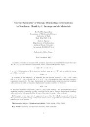
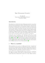
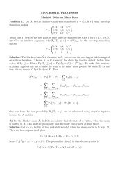
Optimal Stopping and Applications — Free Boundary ProblemsAmg Cox29SinceV z (x) satisfieswhich we can solve to get√where d 1 , d 2 = −µ±β 1 = 1 − β 2 , and that√If we introduce γ =asµ 2 +2λσ 2σ 2µ 2 +2λσ 2σ 2L X f = 1 2 σ2d2 fdx 2 + µdf dx ,12 σ2d2 V zdx 2 + µdV zdx − λV z = 0V z (x) = β 1 e d 1x + β 2 e d 2x. Applying the boundary condition at x = 0, we see thatV z (x) = e d 1x + β 2 (e d 2x − e d 1x )., δ = − µ σ 2 , then γ ≥ −δ ≥ 0, and we can rewrite the solutionV z (x) = e δx [e γx − 2β 2 sinh(γx)] .Applying the second boundary condition, V z (z) = α, we see thatand therefore:β 2 = 1 e γz − αe −δz2 sinh(γz) ,[V z (x) = e δz e γx − sinh(γx) ]sinh(γz) (eγz − αe −δz ) .Note that for x ≤ z, e γz sinh(γx) ≤ e γx sinh(γz), and therefore the expression is positive.If we now differentiate this expression in x, we get[V z(x) ′ = δV z (x) + e δx γe γx − γ cosh(γx) ]sinh(γz) (eγz − αe −δz )and therefore at the right boundary,[V z ′ (z) = δα + eδz γe γz − γ cosh(γz) ]sinh(γz) (eγz − αe −δz ) .If we differentiate this whole expression again with respect to z and simplify, we get:ddz [V ′z (z)] =γ [γ(cosh((δ + γ)z) − α) − δe −δzsinh 2 sinh(γz) ] .(γz)It follows that this expression is non-negative (since γ ≥ −δ ≥ 0), and therefore thatV ′z(z) is increasing as a function of z.This allows us to think of the solutions to the free boundary problem for given z as follows:V ′1(1) ≤ 0: In this case, since the gradient increases as z increases, there exists a uniquez ∗ ≥ 1 such that V z ′ ∗(z∗ ) = 0, and for all z < z ∗ , V z(z) ′ < 0 and for all z > z ∗ ,(z) > 0. This is represented in Figure 1.V ′zPlease e-mail any comments/corrections/questions to: A.M.G.Cox@bath.ac.uk.

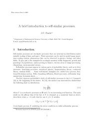
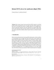
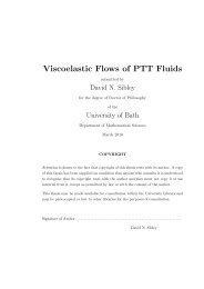
Optimal Stopping and Applications — Free Boundary ProblemsAmg Cox3010.80.60.40.200 0.5 1 1.5 2 2.5 3Figure 1: Possible functions V z (x) for different values of z. In this case, V 1 (1) < 0. Theparameter values are α = 1 , µ = 0.25, λ = 0.1, σ = 1. Note that there is a ‘largest’2function which has V z ′ ∗(z∗ ) = 0.V ′1′(1) > 0: In this case, again, since the gradient increases as z increases, V z (z) > 0 forall z ≥ 1. This is represented in Figure 2.In the first case, where there is a z ∗ ≥ 1 such that V z ′ ∗(z∗ ) = 0, we can deduce that thismust be the only plausible solution to (35)–(38) — any smaller choice of z gives a functionV z (x) (extended to R + with V z (x) = α for x > z) which has a kink at z with left derivativewhich is negative and right derivative zero. Consequently, the value function is (strictly)convex at this point, and V z (X s ) would be a (strict) submartingale at this point, whichis not possible. Conversely, if we choose a z < z ∗ , V z(z) ′ > 0, and the function V z wouldnot remain above the gain function. As a result (see the argument following (35)–(38)),V z ∗(x) is the value function. Note that in this case, z ∗ can be recovered by looking forthe solution to the free-boundary problem: find V, z such thatL X V = λV,V (0) = 1,V (z) = α,V ′ (z) = 0.x ∈ (0, z),Please e-mail any comments/corrections/questions to: A.M.G.Cox@bath.ac.uk.

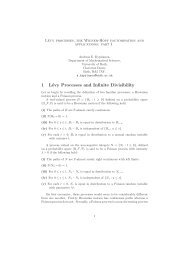
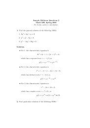
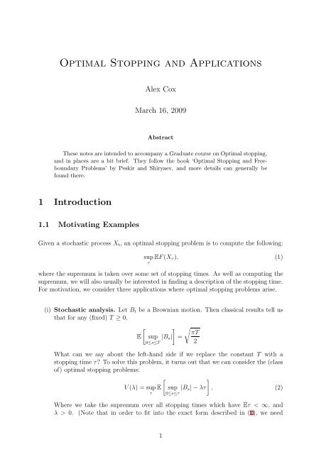
Optimal Stopping and Applications — Free Boundary ProblemsAmg Cox3110.80.60.40.200 0.5 1 1.5 2 2.5 3Figure 2: Possible functions V z (x) for different values of z. In this case, V 1 (1) > 0. Theparameter values are α = 1 , µ = 0.25, λ = 2, σ = 1. Note that there is no function which2has V z ′ ∗(z∗ ) = 0.The final condition in this case being the smooth-fit condition.In the second case, where V ′1(1) > 0, we see again that we cannot take larger values ofz since the resulting value function passes below the value function. It is easy to seehowever that (35)–(38) holds for z ∗ = 1, and this is therefore the optimal choice for thestopping region. In this case, there is no smooth-fit criterion. There are no hard-and-fastrules regarding when there is or is not a smooth-fit principle, but in this example, it is aconsequence of the discontinuity in the gain function. In examples where the gain functionis smoother, one would expect the smooth-fit principle to hold — see Figure 3, where again function G(x) = tanh(x) for x > 0 is used.Please e-mail any comments/corrections/questions to: A.M.G.Cox@bath.ac.uk.

Optimal Stopping and Applications — Free Boundary ProblemsAmg Cox3210.80.60.40.200 0.5 1 1.5 2 2.5 3Figure 3: An alternative payoff function, again exhibiting similar behaviour as above, butthis time a smooth-fit criterion can always be applied.Please e-mail any comments/corrections/questions to: A.M.G.Cox@bath.ac.uk.