A brief introduction to self-similar processes. - Cimat

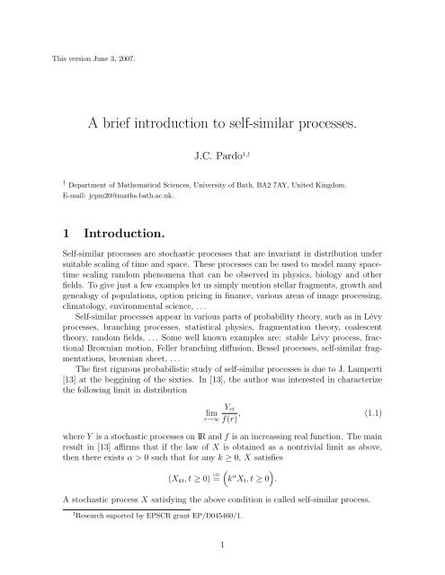
This version June 3, 2007.A brief introduction to self-similar processes.J.C. Pardo 1,†† Department of Mathematical Sciences, University of Bath, BA2 7AY, United Kingdom.E-mail: jcpm20@maths.bath.ac.uk.1 Introduction.Self-similar processes are stochastic processes that are invariant in distribution undersuitable scaling of time and space. These processes can be used to model many spacetimescaling random phenomena that can be observed in physics, biology and otherfields. To give just a few examples let us simply mention stellar fragments, growth andgenealogy of populations, option pricing in finance, various areas of image processing,climatology, environmental science, . . .Self-similar processes appear in various parts of probability theory, such as in Lévyprocesses, branching processes, statistical physics, fragmentation theory, coalescenttheory, random fields, . . . Some well known examples are: stable Lévy process, fractionalBrownian motion, Feller branching diffusion, Bessel processes, self-similar fragmentations,brownian sheet, . . .The first rigurous probabilistic study of self-similar processes is due to J. Lamperti[13] at the beggining of the sixties. In [13], the author was interested in characterizethe following limit in distributionlimr→∞Y rtf(r) , (1.1)where Y is a stochastic processes on IR and f is an increassing real function. The mainresult in [13] affirms that if the law of X is obtained as a nontrivial limit as above,then there exists α > 0 such that for any k ≥ 0, X satisfies(X kt , t ≥ 0) (d)=(k α X t , t ≥ 0A stochastic process X satisfying the above condition is called self-similar process.1 Research suported by EPSCR grant EP/D045460/1.).1

The aim of this note is to survey some remarkable properties of self-similar processes.In particular, we are interested in self-similar processes with independent incrementsor self-similar additive processes. The relation that exist between such class of selfsimilarprocesses, generalized Ornstein-Uhlenbeck processes and a particular class ofLévy processes is proved in detail. We will assume that the reader is related with thetheory of infinitely divisible distributions and Lévy processes.2 Self-similar processes.In this section, we introduce self-similar processes. Some remarkable properties of suchprocesses are studied, as the main result in [13] which characterize the limit distribution(1.1), and the Lamperti representation which gives us a bijection between self-similarprocesses and stationary processes.2.1 Definition and examplesIn the sequel, we consider stochastic processes defined on D, the space of Skorokhod ofcàdlàg paths on [0, ∞) with values in IR. This space is endowed with the J 1 -Skorokhod’stopology. In particular D is a polish space (metric-complete and separable). We denoteby F for the Borel σ-field of the open subsets of D and P will be our reference probabilitymeasure.Recall that a stochastic process (X t , t ≥ 0) is trivial if the law of X t is a dirac measurefor every t > 0.Definition 1 A nontrivial stochastic processes X = (X t , t ≥ 0) taking values on IR issaid to be self-similar if for any a ≥ 0, there exist b(a) ∈ IR such that()(X at , t ≥ 0) (d)= b(a)X t , t ≥ 0 . (2.2)In [13], Lamperti proved that b(a) can be expressed as b(a) = a γ , where γ ≥ 0. Thisfact is not difficult to see it: From the right-continuity at 0 of the process X and theself-similar property (2.2), it follows that the law of X t is not a dirac measure for anyt > 0. Now, we take a, c ≥ 0 and from the self-similar property we get(d)(d)(d)X act = b(ac)X t = b(a)X ct = b(a)b(c)X t .From the above equality in distribution, we get X a n = b n (a)X 1 , n ≥ 1. Since theprocess is nontrivial, the function b is increasing which implies that there exists γ ∈ IR +such that b(a) = a γ .On the other hand, it is clear that if γ > 0, then X 0 = 0 a.s. When γ = 0 then Xis a.s. constant, i.e. X t = X 0 for all t ≥ 0, a.s. Hence the definition of self-similarprocesses becomes:Definition 1’ A nontrivial stochastic processes X = (X t , t ≥ 0) taking values on IR issaid to be self-similar if for any a ≥ 0, there exist γ > 0 such that( )(X at , t ≥ 0) (d)= a γ X t , t ≥ 0 .2

The process X is said to be self-similar of index γ = 0 if it is a.s. constant.In the recent literature, self-similar processes are defined as above but there isa more general way to define them. We refer to the Lectures Notes on self-similarprocesses of Chaumont [6] for a more general definition.Before establishing the main results of this section, we first introduce some importantexamples of self-similar processes.Example 1. Recall that a Lévy process is a stochastic process defined on D withindependent and stationary increments, i.e. if X = (X t , t ≥ 0) is a such process thenfor any t ≥ 0 and s ≥ 0,X t+s − X t is independent of (X u , 0 ≤ u ≤ t),and has the same law as X s . Also recall that the class of all Lévy processes is inone-to-one correspondence with the class of all infinitely divisible distributions.In this example, we are interested in a particular sub-class of infinitely divisible distributions,the well-know stable distributions.Definition 2 Let µ be an infinitely divisible probability measure on IR and ˆµ(z) denotesits characteristic function for z ∈ IR, i.e.∫ˆµ(z) = e i µ(dx), z ∈ IR.IR dThe probability measure µ is said to be stable, if for any a > 0 there are b > 0 andc ∈ IR such that (ˆµ(z)) a= ˆµ(bz)e i , for all z ∈ IR.Moreover, µ is said to be strictly stable, if for any a, there is b > 0 such that) a (ˆµ(z) = ˆµ(bz), for all z ∈ IR.According to Sato [18] (see theorems 14.1, 14.2 and 14.3) the constant b = a 1/α , whereα ∈ (0, 2]. The index α is known as the stability index. In particular, when α = 2 thelaw of µ corresponds to the Gaussian case.Here, we are interested in strictly stable distributions and in all the sequel we may referto them as α-stable. We say that X is a stable Lévy process if X is a Lévy processand the law of X 1 is α-stable. Note that when α = 2, X is proportional to a Brownianmotion.The following proposition shows us that stable Lévy processes are the only selfsimilarprocesses with independent and stationary increments.Proposition 1 Let X be a Lévy process with values in IR and such that X 0 = 0 a.s.The law of X 1 is α-stable if and only if X is self-similar. Moreover, the scaling indexis equal to 1/α.3

Proof: Let ˆµ t (λ) = E(e iλXt ) and suppose that X is a self-similar process of index1/α > 0. From definition 1’, we have that X t = t 1/α X 1 for any t > 0. On the otherhand, since X is a Lévy processes we known thatˆµ t (λ) = (ˆµ 1 (λ) ) t, for all λ ∈ IR,hence (ˆµ 1 (λ) ) t= ˆµ1 (t 1/α λ), which implies that the law of X 1 , denoted by µ 1 , is α-stable.Now, let us suppose that the law of X 1 is α-stable. Since X is a process with independentand stationary increments, it is enough to show that for any t > 0 and a > 0,(d)X at = a 1/α X t . However, ˆµ at (λ) = (ˆµ 1 (λ) ) at= ˆµt1 (a 1/α λ) = ˆµ t (a 1/α λ), which completesthe proof.It is important to note that stable Lévy processes also belong to the class of self-similaradditive processes.Example 2. Another important example is the fractional Brownian motion, which isa self-similar Gaussian process.Definition 3 Let H ∈ (0, 1]. The fractional Brownian motion is a mean-zero Gaussianprocess B (H) = (B (H)t , t ≥ 0) which covariance is given by( )E B (H) = 1 ( (B2 (t2H + s 2H − |t − s| 2H (H)) ) 2)E .B (H)tsNote that when H = 1/2, the process B (1/2) is the standard Brownian motion.1Proposition 2 The fractional Brownian motion B (H)scaling index H.is a self-similar process withProof: From its covariance, it is clear( )E B (H)at B as(H) = 1 ) ( (B ((at) 2H + (as) 2H − (a|t − s|) 2H (H)) ) 2E 12 ( )= a 2H E B (H) .B (H)tsSince B (H) is a Gaussian process, the above equality shows that the processes a H B (H)and (B (H)at , t ≥ 0) have the same law.The fractional Brownian motion (FBM for short) also have stationary increments, thiscan be easily seen using again its covariance and the fact that B (H) is a Gaussianprocess. We also note that when H ≠ 1/2, the FBM is neither a Markov processand nor a semi-martingale. In particular, Ito’s calculus does not work for the FBM.Recently many authors introduce different methods to define a stochastic integral withrespect to the FBM, many of them use the Hölder continuity of the paths of B (H) . Inorder to give some examples, we just mention: the Young integral, Skorokhod integral(via Malliavin Calculus), rough paths, . . .4

Self-similar processes with stationary increments is probably the most studied classof self-similar processes (thanks to the FBM). The stationarity of the increments allowus to obtain nice properties of their trajectories. In this note we will not study suchclass of processes, we refer to the monographe of Embrechts and Maejima [8] andChaumont [6] for a deep discussion on this topic.Example 3. Now let us mention an example of self-similar processes with independentincrements (or self-similar additive processes) which does not have stationaryincrements, i.e. not a stable Lévy process.Let X be a self-similar Markov process with no positive jumps taking values in IR +and starting from x ≥ 0. From the Markov property, self-similarity and the absence ofpositive jumps, it is clear that the first passage timey ↦−→ inf { t : X t = y } ,is an increasing self-similar process with independent increments. Self-similar processeswith independent increments are also called as processes of class L and have an importantconnection with generalized Ornstein-Uhlenbeck processes and Lévy processes.Such connection will be studied in section 3.2.2 Convergence theorems and “first” Lamperti representation.Self-similar processes are obtained as weak limits of rescaled stochastic processes. Thisphenomena is well-known for stable Lévy processes and branching processes since longtime ago (see for instance Lamperti [14, 15] and Grimvall [10]) and recently remarkedfor Lévy trees [7] and fragmentation processes [3, 4].Here, we are interested in sequences (X n ) of random variables which converge in lawafter a change of location and scale. That is, there exist centring constants b n andnorming constants a n > 0 such thatX n − b na n(d)−→ X, (2.3)where “ −→” (d)means convergence in distribution or in law. Recall that two randomvariables X and Y are said to belong to the same type if they have the same law afterchange of location and scale, i.e. ifY (d)= uX + v, for some u > 0 and v ∈ IR d ,where “ (d)=” means equality in law.The following result knonw as Convergence of Types Lemma means in particular that,to whitin type, the convergence (2.3) cannot hold in two differents ways. Such resultwill not be proved here but its proof can be found in Gnedenko and Kolmogorov [9] orin chapter 1 of [6].5

Lemma 1 Let X, Y and (X n ) a.s. finite random variables taking values in IR. Wesuppose that the law of Y is nontrivial. If there exist real sequences a n > 0, α n > 0,b n ∈ IR and β n ∈ IR verifyingthenX n − b na n(d)−→ Xa nα n→ u ∈ (0, ∞)andandX n − β nα n(d)−→ Y, as n → ∞, (2.4)b n − β nα n→ v ∈ IR, as n → ∞. (2.5)Moreover if the relations in (2.4) and (2.5) are satisfied, u and v are the unique constantssuch that Y (d)= uX + v.Regularly varying functions are so important in the theory of self-similar processessince they appear in their construction (see Theorem 2 below). Here, we will only recalltheir definition and some important properties which will be needed for the proof ofTheorem 2. We refer to the monographe of Bingham et al. [5] for a deep study on thissubject.Definition 4 A function L : IR + → IR is said to be a slowly varying function in +∞,if for any a > 0,L(ax)limx→+∞ L(x) = 1.Moreover, a function F : IR + → IR is said to be a regularly varying function of indexβ in +∞, if for any a > 0,F (ax)limx→+∞ F (x) = aβ .It is not difficult to see that if F : IR + → IR is a regularly varying function of index β,then there exists L a slowly varying function such thatF (x) ∼ x β L(x), as x → +∞.The following result is an important characterization of regularly varying functions.Theorem 1 Let F : IR + → IR be a Lebesgue measurable function. If F satisfiesF (ax)limx→+∞ F (x)then F is a regularly varying function.∈ (0, ∞), for any a > 0,Proof: LetFor b > 0, we haveF (ax)G(a) = lim , for a > 0.x→∞ F (x)G(ab) = limx→∞F (abx)F (x)F (abx)= limx→∞ F (bx)6F (bx)F (x) = G(a)G(b).

The function G : (0, ∞) → (0, ∞) is multiplicative. Since G is measurable andmultiplicative then there exists some β ∈ IR such that G(a) = a β . Finally, letL(x) = F (x)/x β . Therefore for every λ > 0,and the result follows.L(λx)limx→∞ L(x) = 1,The next result, due to Lamperti [13], connects self-similar processes with limittheorems.Theorem 2 Let Y be a IR-valued stochastic process. If there exist a process X suchthat X 1 is nontrivial and f a Borel function satisfying that lim r→∞ f(r) = ∞ andY rtf(r) −→ X t as r → ∞, (2.6)holds in the sense of finite-dimensional distributions, then the process X is self-similarwith index γ > 0. Moreover, f is a regularly varying functions of index γ.Conversely, any self-similar process X of strictely positive index may be obtained asthe limit in law (2.6).Proof: Assume that (2.6) is satisfied and choose a real sequence (r n ) which divergetowards +∞. We first prove that f is a regularly varying function. From (2.6), wededuce that for t > 0 and any y ∈ IR()P Y rn ≤ f(r n )y −→ P(X 1 ≤ y),()P Y rn ≤ f(r n t)y −→ P(X 1/t ≤ y),as n goes to +∞. Hence from Lemma 1 and the fact that X 1 is nontrivial, the limit off(r n t)/f(r n ), as n goes to +∞, exists and is strictely positive. Note that for t > 0 theabove limit holds for any sequence which diverge towards +∞. Then the limit existstaking r → ∞. By Theorem 1, the function f is regularly varying and since f divergetowards +∞, its index γ is positive or zero. Since the function f diverges towards +∞and taking t = 0 in (2.6), it is clear that X 0 = 0 a.s.Now, we will prove the self-similar property of the process X. Let a > 0, (t 1 , . . . , t n ) ∈IR n + and (x 1 , . . . , x n ) a continuity point for the distribution function of (X at1 , . . . , X atn )such that (a −γ x 1 , . . . , a −γ x n ) is a continuity point for the distribution function of(X t1 , . . . , X tn ) as well. Then from (2.6) we have(lim P Yrat1r→+∞ f(r) ≤ x 1, . . . , Y )rat nf(r) ≤ x n = P(X at1 ≤ x 1 , . . . , X atn ≤ x n ).The distribution function of the left hand-side of the above equality can be written as()Y rat1Pf(ar) ≤ f(r)f(ar) x 1, . . . , Y rat nf(ar) ≤ f(r)f(ar) x n .7

Hence, taking the limit when r goes to +∞ we obtain that the above distributionfunction converge towards)P(X t1 ≤ a −γ x 1 , . . . , X tn ≤ a −γ x n ,which proves that the process X is self-similar. The case where γ = 0 is not possiblesince we are assuming that the process X is nontrivial.The second part of the proof is evident. Let X be a self-similar process of index γ > 0.In order to obtain (2.6), it is enough to take Y = X and f(r) = r γ and then apply thescaling property of X.There exists a version of this theorem for discrete-time stochastic processes. In orderto establish such result, we first recall the definition of regularly varying sequence: asequence a(n) is regularly varying if there exists γ ∈ IR such that for all t > 0a(nt)limn→+∞ a(n) = tγ .Theorem 3 Let (Y n ) be a sequence of a.s. finites random variables taking values inIR. If there exist a process X a.s. finite such that X 1 is nontrivial and a(n) a sequencesatisfying that lim n→+∞ a(n) = +∞ andY [nt]a(n) −→ X t as n → +∞, (2.7)holds in the sense of finite-dimensional distributions, then the process X is self-similarwith index γ > 0. Moreover, a(n) is a regularly varying sequence of index γ.Conversely, if a self-similar process X of strictely positive index may be obtained asthe limit in law (2.7).The idea of the proof of the above theorem is basically the same as that of thecontinuous version, but note that it requires additional results on regularly varyingsequences. We refer to section 8.5 of the monographe of Bingham, Goldie and Teugels[5] for its proof.Now, we introduce the “first” Lamperti representation. In this direction, we recallthe definition of stationary process.Definition 5 A stochastic process (Y t , t ∈ IR) is said to be stationary if its law remainsequal regardless of any shift, θ t for any t, in time, i.e. if it verifies the following identityin law(Y s , s ∈ IR) (d)= (Y t+s , s ∈ IR) (def)= Y ◦ θ t , for all t ∈ IR.Proposition 3 (“First” Lamperti representation) If (Y t , t ∈ IR) is an stationaryprocess, then for all γ > 0 the process defined by(def)X t = t γ Y log t , for t > 0 and X 0 = 0,8

is a self-similar process of index γ > 0. Conversely, if the process X is self-similar ofindex γ > 0 and such that X 0 = 0, then the processus defined byis stationary.(Y t , t ∈ IR) (def)= ( e −γt X e t, t ∈ IR ) ,Proof: Let n ≥ 1 and β 1 , . . . , β n real numbers. Let us suppose that the process Y isstationary, then for any a, γ > 0 and t 1 , ..., t p ∈ IR + ,n∑n∑n∑n∑β j X atj = β j a γ t γ j Y (d)log a+log t j= β j a γ t γ j Y log t j= β j a γ X tj ,j=1j=1proving that X is self-similar of index γ.Conversely, if X is self-similar of index γ > 0, then for any h > 0 and t 1 , ..., t p ∈ IR + ,n∑n∑n∑n∑β j Y tj +h = β j e −γt je −γh (d)X et j e= β h j e −γt jX et j ) = β j Y tj ,j=1j=1proving that Y is stationary.j=1j=1j=1j=1The stationary process related with a self-similar process X by the “first” Lampertirepresentation is called some times as the Ornstein-Uhlenbeck process associatedto X. This name comes from the known Ornstein-Uhlenbeck process which is definedby Y = (e −t/2 B (1/2)e, t ∈ IR) where B (1/2) is the standard Brownian motion.tIt is important to note that the self-similar (or scaling) property by its self does notallow us to determine the distributions of self-similar processes. Actually it was noted in[1] that even in the case when self-similar processes have stationary increments thereis no simple characterization of the possible families of their marginal distributions.This is not the case for self-similar processes with independent increments. We willsee in the next section that in fact self-similar additive processes is related to the classof self-decomposable distribution as Lévy processes is related to the class of infinitelydivisible distributions.3 Self-similar additive processes.This section introduce the laws of class L and self-similar additive processes (ssap forshort), i.e. self-similar processes with independent increments. The connection of thelaws of class L and ssap is described. Self-similar additive processes are related to aparticular class of Lévy processes, such connection is also described here. In particularwe will obtain that the stationary process Y related with a ssap by the firs Lampertirepresentation is the solution of the Ornstein-Uhlenbeck equation associated with aBackground Driving Lévy process ξdY t = −γY t dt + dξ t ,with initial condition Y 0 = H is an independent r.v. of ξ.9

3.1 Laws of Class L and self-decomposable laws.Roughly speaking a random variable has a distribution of class L if the random variablehas the same distribution as the limit of some normalized sequence of sums of independentrandom variables. More precisely, consider a sequence (X n , n ≥ 1) of independentrandom variables on IR and let S n = ∑ nk=1 X k denote their sum. Suppose that thereexist two sequences c(n) ∈ IR and b(n) > 0 such that for every ɛ > 0lim max P(b n|X k | > ɛ) = 0, (3.8)n→∞ 1≤k≤nand the distribution of b(n)S n + c(n) converges to the distribution of some randomvariable X on IR. The random variable X is said to be on the class L.From Theorem 9.3 in Sato [18] and condition (3.8), we deduce that the distribution ofany random variable in the class L is infinitely divisible. The class L have been studiedby many authors, the oldest of these is due to Levy [16]. Khintchine [12] seems to bethe first to use the name “Class L”. Well-known examples of laws of class L are theGaussian and stable distributions (see Theorem 5 below).The following definition is an extension of the notion of stable distributions.Definition 6 Let µ be a probability measure on IR and ˆµ denotes its characteristicfunction. We say that µ is self-decomposable if for any b > 1, there is a probabilitymeasure ρ b on IR such thatˆµ(z) = ˆµ(bz)ˆρ(z),z ∈ IR,where ˆρ denotes the characteristic function of ρ b .In terms of random variables this definition becomes: a random variable X is said tobe self-decomposable if for any constant c ∈ (0, 1) there exists an independent randomvariable, say X (c) such thatX (d)= cX + X (c) .In other words, a random varialbe is self-decomposable if it has the same distributionas the sum of a scaled down version of itself and an independent residual random variable.An important example of such class of distributions are stable distribution.The following theorem shows that a random variable has a distribution of class Lif and only if the law of the random variable is self-decomposable. The proof of thistheorem can be found in Sato [18] (Theorem 15.3).Theorem 4 Let (X n , n ≥ 1) be a sequence of independent random variables on IR andS n denote their sum as above. Let X be a random variable with values on IR which hasa distribution of class L, then X is self-decomposable.Conversely, for any self-decomposable random variable X on IR we can find a sequence(X n , n ≥ 1) of independent random variables on IR and two sequences a(n) ∈ IR andb(n) > 0 satisfying that the distribution of b(n)S n + a(n), where S n is defined as before,converge to the distribution of X and (3.8).10

The above result give us automatically that the class of self-decomposable distributionsis a sub-class of infinitely divisible distributions. In particular, if µ is self-decomposableits Lévy measure has the following structureΠ(dx) = k(x)|x| dx,where k is a positive measurable function increasing on (−∞, 0) and decreasing on(0, ∞), i.e that the Levy measure Π is unimodal with mode 0. Yamazato [20] provedthat self-decomposable laws in IR have the unimodal property, i.e. that their densitiesare unimodal.The following limit theorem gives a characterization of stable distributions as in the caseof self-decomposable distributions. In particular, we obtain that stable distributionsare self-decomposable and unimodal.Theorem 5 A probability measure µ on IR is stable if and only if there are a randomwalk (S n , n ≥ 1) and a sequence b(n) > 0 such that the distribution of b(n)S n convergesto µ, as n goes to ∞.Proof: Suppose that the distribution of b(n)S n converges to µ and that µ is nontrivial.For any k ∈ IN, consider∑k−1(b(n)S kn = b(n) ( ) )S (j+1)n − S jn .j=0The distribution of the right-hand side tends to µ ∗n as n goes to ∞, while the distributionof b(kn)S kn converges to µ. From Lemma 1, there is b > 0 such that ˆµ(z) k = ˆµ(bz).This implies that µ is stable.Conversely, let µ be stable. Choose a random walk (S n , n ≥ 1) with step distributionequal to µ. The stability implies that b(n)S n has distribution µ if b n > 0 is suitablechosen.It is known that a probability measure µ with support in IR + is infinitely divisibleif and only if its Laplace transform has the form∫ ∞{ ∫ ∞(e −ux µ(dx) = exp −au −) }1 − e−uxν(dx) ,0where a ≥ 0 and the measure ν is defined on (0, ∞) and satisfies∫ ∞0(1 ∧ x)ν(dx) < ∞.Then the Lévy measure of a self-decomposable distribution with support in IR + hasthe form ν(dx) = k(x)/x. The asymptotic of the densities of self-decomposable distributionswith support in IR + at 0 satisfy a particular behaviour when the drift is 0. Inparticular such densities are regularly varying at 0.011

Theorem 6 Let µ be a self-decomposable distribution on IR + with k-function k(x)satisfying c = k(0+) < ∞, and let∫ ∞{ ∫ ∞(e −ux µ(dx) = exp −) }1 − e−ux k(x)x dx .0Define{∫ 1L(x) = exp (c − k(y)) dy }, x > 0.xyThen the density f(x) of µ satisfiesf(x) ∼0KΓ(c) xc−1 L(x), as x → 0,where K is the constant given by{ ∫ 1K = exp c (e −x − 1) dx ∫ ∞x + (ce −x − k(x)) dx x0Proof: First we prove that L is slowly varying function at 0 for any λ ∈ (0, 1),{∫L(λx)xL(x) = exp (c − k(y)) dy } {∫ 1= exp (c − k(xy)) dy },yyλxwhich goes to 1 as x tends to 0.Now, let us show that∫ ∞We first observe that ∫ ∞and that∫ 1/u00e −ux µ(dx) ∼ Ku −c L(1/u), as u → ∞.1(e −ux − 1 ) k(x)x dx = ∫ 11/u(e −ux − 1 ) ∫k(x)∞xdx → − 101λk(x)xdx,(e −x − 1 ) k(x/u)dx → −cx1/u∫ ∞1}.(e −x − 1 ) dxxas u goes to ∞. On the other hand,∫ 1(e −ux − 1 ) ∫k(x)1x dx + c log u − log L(1/u) = −ux k(x)exdx=∫ u1−x k(x/u)e dx → cx∫ ∞1e −x dx , as u → ∞.xHence,∫ ∞e −ux µ(dx)0→ K, as u → ∞.u c L(1/u)From Karamata’s Tauberian Theorem (see for instance Theorem 1.7.1 in [5]), we obtainthatµ ( [0, x) ) K∼Γ(c + 1) xc L(x) as x → 0.Since the density of µ is monotone in a right neighborhood of the origin, the monotonedensity theorem (see for instance Theorem 1.7.2 in [5]), give us the desired result.12

3.3 Generalized Ornstein-Uhlenbeck processes.The aim of this section is to establish a representation of self-similar additive processeswith respect to a particular class of Lévy processes. In order to do so, we first introducesome properties of stochastic integration of continuous functions of locally boundedvariation with respect to a given Lévy process.Recall that for all t > 0, a right continuous function g which is of bounded variationinduces a signed measure µ on µ([0, t], B([0, t])):µ((a, b]) = g(b) − g(a) for 0 ≤ a < b ≤ t and µ({0}) = 0.Note that the variation |µ| of µ is the measure associated with the variation |g| of g.If f ∈ L(|µ|), then the Lebesgue-Stieltjes integral of f with respect to g over [0, t], forall t > 0, is defined by∫∫∫∫f(s)dg(s) (def)= fdµ and∣ f(s)dg(s)∣ ≤ |f|d|µ|.[0,t][0,t]If f is a continuous function, then the Riemman-Stieltjes integral of f with respect tog on [0, t] is well defined and equals the Lebesgue-Stieltjes integral, i.e.,∫[0,t]f(s)dg(s) = limn→∞p n∑k=1[0,t][0,t]f(t n i−1) ( g(t n i ) − g(t n i−1) ) , (3.9)for any sequence of partitions 0 = t n 0 < t n 1 < · · · < t n p n= t of [0, t] where max |t n k − tn k−1 |tends to 0 as n goes to ∞. On the other hand, if g is continuous as well as being ofbounded variation then the Lebesgue-Stieltjes integral of f with respect to g is alsogiven by (3.9) when f is a càdlàg function. This last property will give us the followinglemma.Lemma 2 Let ξ = (ξ t , t ≥ 0) be a càdlàg process on IR and A = (A s , s ≥ 0) acontinuous process of bounded variation. Then the stochastic integral of A with respectto ξ on (t 0 , t] defined bymakes sense.∫ t(def)A s dξ s = A t ξ t − A t0 ξ t0 −t 0∫ tt 0ξ s− dA s ,Now, we suppose that the process A is a deterministic function of bounded variation,hence the following corollary follows from the definition of the Riemman-Stieltjesintegral (3.9).Corollary 1 Let ξ = (ξ t , t ≥ 0) be an adapted càdlàg process on IR and f a continuousfunction of bounded variation. Then, the process t ↦→ ∫ tt 0f(s)dξ s is càdlàg, progressivelymeasurable and adapted with respect to the filtration of ξ.If ξ is an additive process, then the process t ↦→ ∫ tt 0f(s)dξ s is also additive.14

If ξ is a Lévy process with characteristic exponent Φ, then ∫ tt 0f(s)dξ s is an infinitelydivisible random variable with characteristic exponent ΨΨ(t) =∫ tt 0Φ(tf(s))ds,t ∈ IR.In particular, if Π is the Lévy measure of ξ, the Lévy mesure M t (dx) of ∫ t0 e−s dξ s isgiven byM t (dx) =∫ t0Π(e s dx)ds.Let Hbe a random variable on IR and ξ a Lévy process which is independent of H.Given c ∈ IR, consider the equationY t = H + ξ t − c∫ t0Y s ds, t ≥ 0. (3.10)A stochastic process Y = (Y t , t ≥ 0) is said to be a solution of (3.10) if Y is càdlàg andsatisfies (3.10) a.s.Proposition 5 The equation (3.10) has an almost surely unique solution Y and, almostsurely,∫ tY t = e −ct H + e −ct e cs dξ s , t ≥ 0. (3.11)Proof: From lemma 2 and (3.10), we havee ct Y t = H + c= H + c= H +∫ t0∫ t0∫ t00e cs Y s ds +e cs Y s ds +e cs dξ s ,∫ t0∫ t0e cs dY se cs dξ s − c∫ t0e cs Y s dswhich proves that the process Y defined by (3.11) is a unique solution of (3.10).The next result shows that the solution of (3.10) is an homogeneous Markov process.Proposition 6 The process Y defined by (3.11) is an homogeneous Markov processstarting from x with semi-group P t (z, dy), infinitely divisible and satisfying∫ ∞−∞{e iλy P t (z, dy) = exp ie −ct λz +∫ t0}Φ(e −cs λ)ds ,where Φ is the characteristic exponent of the Levy process ξ in (3.11).15

Proof: From (3.11) we have for every s ∈ [0, t],∫ tY t = e −c(t−s) Y s + e −ct e cu dξ u .Corollary 1 give us that the integral of the right-hand side of the above equality isindependent of (Y u , 0 ≤ u ≤ s) and therefore the Markov property follows.Again from corollary 1 is clear that the law of Y t is infinitely divisible and with characteristicexponentΨ(λ) = iλe −ct x +which concludes the proof.∫ t0Φ(λe −c(t−u) )du = iλe −ct x +s∫ t0Φ(λe −cs )ds,The process Y defined by (3.11) is called Ornstein-Uhlenbeck process driven byξ with initial state H and parameter c ∈ IR. The following result deals with limitdistributions of Ornstein-Uhlenbeck processes as t goes to 0. In particular, it showsthat an Ornstein-Uhlenbeck process has a limit distributions when the backgrounddriving Lévy process does not have big jumps.Theorem 7 Let c > 0 be fixed.i) Let ξ be the background driving Lévy of Y the Ornstein-Uhlenbeck process definedby (3.11) starting from x. Assume that∫log |x|Π(dx) < ∞, (3.12){|x|>2}where Π is the Lévy measure of ξ. Then the law of Y t converge towards µ aself-decomposable law as t goes to ∞. Moreover, the characteristic function of µis given by{∫ ∞}ˆµ(λ) = exp Φ(e −cs λ)ds , (3.13)0where Φ is the characteristic exponent of ξ 1 .ii) Let µ be a self-decomposable, then there exist a Lévy process ξ which Lévy measuresatisfies (3.12) such that µ satisfies (3.13) for the Ornstein-Uhlembeck processgenerated by ξ and a constant c.iii) If we assume that∫{|x|>2}log |x|Π(dx) = ∞.Then the law of Y t does not tend to any distribution as t goes to ∞.16

We will not prove the above result. We refer to Theorem 17.5 in Sato [18] for a proof.The limit distribution µ of an Ornstein-Uhlenbeck process is self-decomposable andfrom our previous sub-section, we know that there is a self-similar additive processrelated to µ then a natural question is: could we identify one process from another?The following theorem will give us an affirmative answer to this question.Before establishing our next result, we recall that Wolfe [19] and Jurek and Vervaat[11] showed that the distribution of a random variable X 1 is self-decomposable if andonly if(d)X 1 =∫ ∞0e −s dξ s , (3.14)where ξ = (ξ t , t ≥ 0) is a Lévy process satisfying that E ( log(1 ∨ |ξ s |) ) < ∞ for all s.The process is called the background driving Lévy process of X 1 . We denote by Υ theclass of Levy processes ξ satisfying that(E)log(1 ∨ |ξ s |) < ∞ for all s ≥ 0.Note that from theorem 7, the distribution of X 1 is the limit distribution of a Ornstein-Uhlenbeck process driven by ξ and with parameter 1.Theorem 8 Let X be a self-similar additive process with index γ > 0.following formulasThen, theξ (−)t(def)=∫ 1dX rand ξ (+)e r −t γ t(def)=∫ e t1dX rr γdefine two independent and identically distributed Lévy process ξ (−) = (ξ (−)t , t ≥ 0) andξ (+) = (ξ (+)t , t ≥ 0) which belongs to Υ and from which X can be recovered by⎧ ∫ ∞⎪⎨ e −tγ dξ (−)t if 0 ≤ r ≤ 1,X r =⎪⎩ X 1 +log(1/r)∫ log(r)0e tγ dξ (+)t if r ≥ 1,(3.15)where the law of X 1 is a self-decomposable distribution. In particular the BDLP of X 1is (ξ (−)t/γ , t ≥ 0). Conversely, given a BDLP (ξ t, t ≥ 0) of the class Υ associated witha self-decomposable distribution of X 1 via (3.14), a corresponding self-similar additiveprocess can be constructed by (3.15) from two independent copies (ξ (−)t , t ≥ 0) and(ξ (+)t , t ≥ 0) of (ξ tγ , t ≥ 0).Proof: From Corollary 1, it is clear that the processes (ξ (−)t , t ≥ 0) and (ξ (+)t , t ≥ 0) areindependent and that each of these processes has independent increments. In order toshow that both processes are Lévy processes, it just remains to check that they havestationary increments. Let t, h ≥ 0, from the scaling property of X, we get∫ e −t ∫ξ (−)t+h − dX 1∫r d v X 1e ξ(−) t ==−t v (d) dX v=e r −(t+h) γ e (e −h −t v) γ e v −h γ17= ξ (−)h .

The corresponding result for ξ (+) follows from similar arguments, or by writingξ (+)t =∫ 1e −t d(−X 1/v )v −γ ,and appealing to the previous case with X v replaced by −X 1/v . Since both ξ (−) and ξ (+)have independent increments, to show that they are identically distributed it sufficesto show that they have the same one-dimensional distributions. But for each fixed tand the scaling property of X,∫ 1e −t dX rr γ =In order to obtain (3.15), writeso that∫ ∞0ξ (−)te −vγ ξ (−)v∫ e t1∫d v X e te −t r (d) dX r=(e −t r) γ 1 r . γ∫ td v X e −v= − ,0 e −vγ= −∫ ∞0d v X e −v = X 1This is (3.15) for r = 1 and the general case is obtained by a similar claculation.Finally, the converse assertion is easily checked.Recall that from the “first” Lamperti representation, we know that there exist astationary process (Y t , t ∈ IR) such thatY u = e −uγ X e u.If we compare this representation to (3.15) of a self-similar additive process of indexγ > 0, in terms of the Lévy process ξ (+) , we see that for r ≥ 1so that, with r = e u for u ≥ 0,r γ Y log(r) = Y 0 +Y u = e −uγ (Y 0 +∫ log(r)0∫ u0e tγ dξ (+)t ,)e tγ dξ (+)t .Togheter with similar considerations for (Y −u , u ≥ 0), we deduce the following:Corollary 2 The “first” Lamperti representation (Y u , u ∈ IR) of a self-similar additiveprocess X with index γ > 0 is such that for the two independent Lévy processes ξ (+)and ξ (−) introduced in Theorem 8:i) (Y u , u ≥ 0) is the Ornstein-Uhlenbeck process driven by ξ (+) with initial state X 1and parameter c = γ, andi) (Y −u , u ≥ 0) is the Ornstein-Uhlenbeck process driven by −ξ (−) with initial stateX 1 and parameter c = −γ.18

References[1] O.E Barndorff-Nielsen and V. Pérez-Abreu. Stationary and self-similarprocesses driven by Lévy processes. Stochastic Process. Appl. 84, no. 2, 357–369,(1999).[2] J. Bertoin: Lévy processes. Cambridge University Press, Cambridge, (1996).[3] J. Bertoin: Self-similar fragmentations.Ann. I. H. Poncaré, 38, no. 3, 319–340,(2002).[4] J. Bertoin: Random Fragmentation and Coagulation processes. Cambridge UniversityPress, Cambridge, (2006).[5] N. Bingham, C.M. Goldie and J.L. Teugels: Regular variation. CambridgeUniversity Press, Cambridge, 1989.[6] L. Chaumont: Introduction aux processus auto-similaires. Cours du DEA deProabilités et Applications. Université de Paris VI. (2006).[7] T. Duquesne and J.F. Le Gall: Random trees, Lévy processes and spatialbranching processes. Astérisque 281. Paris: Société Mathématique de France. vi,(2002).[8] P. Embrechts and M. Maejima: Self-similar processes. Princeton UniversityPress, Princeton, NJ, (2002).[9] B.V. Gnedenko and A.N. Kolmogorov: Limit theorems for sums of independentrandom variables. Addison-Wesley, Cambridge, Mass., (1954).[10] A. Grimvall: On the convergence of sequences of branching processes. Ann.Probab., 2, 1027–1045, (1974).[11] Z.J. Jurek and W. Vervaat: An integral representation for self-decomposableBanach space valued random variables. Z. Wahrscheinlichkeitstheorie und Verw.Gebiete, 62, 247–262, (1983). 205–225, (1972).[12] A.Y. Khintchine: Limit laws of sum of independent random variables, ONTI,Moscu, (1938).[13] J. Lamperti: Semi-stable stochastic processes. Trans. Amer. Math. Soc., 104,62–78, (1962).[14] J. Lamperti: The limit of a sequence of branching processes. Z. Wahrscheinlichkeitstheorieund Verw. Gebiete, 7, 271–288, (1967).[15] J. Lamperti: Limiting distributions of branching processes. Proc. Fifth BerkeleySymp. Math. Statist. Probab., 2, 225–241. University California Press, Berkeley(1967).19

[16] P.Lévy: Théorie de l’addition des variables aléatoires. Gauthier-Villars, Paris,(1937).[17] K. Sato: Self-similar processes with independent increments. Probab. TheoryRelated Fields, 89, 285-300, (1991).[18] K. Sato: Lévy processes and infinitely divisible distributions. Cambridge UniversityPress, Cambridge, (1999).[19] S.J. Wolfe: On a continuous analogue of the stochastic difference equationX n = ρX n−1 + B n . Stochastic Process. Appl. 12, no. 3, 301–312, (1982).[20] M. Yamazato: unimodality of infinitely divisible distributions functions of classL. Ann. Probab., 6, 523–531, (1978).20