Smolders - AMESim Intro.pdf - vecom
Smolders - AMESim Intro.pdf - vecom
Smolders - AMESim Intro.pdf - vecom
- No tags were found...

You also want an ePaper? Increase the reach of your titles
YUMPU automatically turns print PDFs into web optimized ePapers that Google loves.
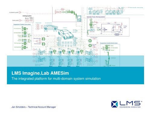
LMS Imagine.Lab <strong>AMESim</strong>The integrated platform for multi-domain system simulationJan <strong>Smolders</strong> – Technical Account Manager
Agenda1. System Simulation2. LMS Imagine.Lab <strong>AMESim</strong>3. <strong>AMESim</strong> Basic Principles4. <strong>AMESim</strong> Workflow5. <strong>AMESim</strong> Analysis Tools2 copyright LMS International - 2010
3 copyright LMS International - 2010System Simulation
<strong>Intro</strong>duction to SystemsWhat is a System?A groupofmulti-domain / multi-physics componentsinteracting togetherSystems have structure, defined by parts and their compositionSystems have behavior, which involves inputs, processing and outputs of material, energy or informationSystems have interconnectivity: the various parts have functional and structural relationships4 copyright LMS International - 2010
What is a system? ExamplesWashing MachineControlElectricHydraulicMechanicThermal5 copyright LMS International - 2010
What is a system? ExamplesElectro-hydraulic power steering systemControlElectricHydraulicMechanic6 copyright LMS International - 2010
What is System Simulation? Usual design issues : Is the electric motor powerful enough? What is the time response of the system? What maximum pressure can be reach? Is there any risk of vibration? How to optimize the control design? Key words : Multi-physics with power exchange Dynamic system (function of time) Physical system model = Plant model<strong>AMESim</strong> plant modelControl Electric Hydraulic Mechanic7 copyright LMS International - 2010
Abstraction Level - Power Steering Example Power steering example Can we build the complete system model with a CADbasedsoftware? No, since we have no CAD at this stage of designCan we simulate it within an acceptable simulation(computational) time making use of 3D only methods? No, no 3D software is able to do that ModelWe need another approach to :• Pre-design such systems• Choose an architecture (hydraulic, electrohydraulic,electric)• Assess key functions of the system8 copyright LMS International - 2010
Abstraction Level – Equations – Representation Equations are usually written as time dependent Computing state derivative of variables to assess transient evolution Equations are represented by readable objects (icons)EquationsPhysical IconRepresentationMechanicsM*dx/dt²= F−Rdx/dt−Kxs22+ 2⋅z ⋅ω⋅ s + ω = 0nnElectricU = R * IdU / dt =I/ CHydraulicsQ = displ * ΩT = displ * ∆PAnd many other physical domains…9 copyright LMS International - 2010
Power Flow within dynamic system System simulation is linked to the power flow and power conservation within a dynamic system Each power network can be modeled using different physics with gates for sub-system connectionsYou are manipulating equationsnot drawing a circuit !ElectricpowernetworkHydraulicpowernetworkMechanicpowernetworkPower flow10 copyright LMS International - 2010
Imagine.Lab <strong>AMESim</strong><strong>Intro</strong>duction11 copyright LMS International - 2010
Why <strong>AMESim</strong> for Multi-Domain System Simulation? Simulation of the complete system Description of physical phenomena based onfew “macroscopic” parameters Multi-domain / Multi-level approach The simulation model is an assembly ofcomponents Components are described with analytical ortabulated models We are looking for static/dynamic responses(time & frequency domains)BrakingPower steeringSuspension12 copyright LMS International - 2010
Our Vision As a supplier: to be able to As a manufacturer: to be able tosimulate and validate components simulate the integration of all suppliersas soon as possible, to provide components and systems in order tomodels for their final customer match the product functionsenvironmentspecifications and validate design choice13 copyright LMS International - 2010Hence the need for aSystem Simulation Mock-Up!
LMS Imagine.Lab <strong>AMESim</strong>: positioningSimulationDetail LevelRequirementsSystemPrototypeFunctionalSub-systemSystemComponentLMSImagine.Lab<strong>AMESim</strong>ComponentLMS Virtual.LabTime14 copyright LMS International - 2010
Positioning in CAx world3D simulationFEMMBSCONTROLCFDMECHANICSHYDRAULICSCONTROL1D system simulationLMS Imagine.Lab <strong>AMESim</strong>PNEUMATICSPOWER ELECTRONICSTHERMALMAGNETIC15 copyright LMS International - 2010
LMS Imagine.Lab Libraries>30 libraries including>4000 Multi-domainModelsHydraulic & PneumaticAutomotive, Aerospace,Off-highway relatedHydraulicsControlControl systems,Real Time, SiL – HilMechanical1D mechanical system,TransmissionVehicle DynamicsThermalVehicle Thermal Management,Cooling & A/C SystemEnvironmental ControlEngineEngine Control, HybridCombustion, Air PathEnergyFuel Cell, Battery, PowerGenerationElectromechanicalElectromechanicalComponents & Networks16 copyright LMS International - 2010
LMS Imagine.Lab <strong>AMESim</strong> SuiteCreate Simulate Capitalize DeployAMESet<strong>AMESim</strong> AMECustom AMERun•Development of new•Modeling•Libraries management•Run onlycomponents•Simulation•Model Packaging•Parametric studies•AnalysisUser expertiseStarting PointUser numberExpertise Deployment17 copyright LMS International - 2010
Solutions for several industriesPowertrainChassisAviation & AerospaceFluids SystemsElectromechanicalEnergyLMS Imagine.Lab <strong>AMESim</strong> PlatformCAE connexions Pre/Post processing Analysis tools Optimization Modelica18 copyright LMS International - 2010
LMS Imagine.Lab <strong>AMESim</strong>, an Open Platform with…CFDCFXMBSLMS Virtual.LabMotionEMControlReal TimePIDOOPTIMUS19 copyright LMS International - 2010
LMS Imagine.Lab <strong>AMESim</strong>: 4 Basic PillarsReady-to-Use Physical ComponentsApplication-Specific Tools & SolutionsELECTRICALFLUIDSTHERMALMECHANICALOver 4,000 multi-physics component modelsTransmissionInternal Combustion EngineVehicle DynamicsAero SystemsThermal ManagementElectrical SystemsThermo-fluids ComponentsOpen System Integration PlatformIntegrated System Data ManagementInteroperabilityUser DefinedFunctionsDept.Dept.Dept.Supplier20 copyright LMS International - 2010
LMS Imagine References (not complete)Automotive - TrucksBMWChryslerDAFFiatFordGMHondaHyundaiIT&ENissanPorschePSARenaultTataToyotaVolvoF1 TeamFerrariMercedes MotorsportToyota MotorsportToro RossoDiesel EngineCRT AGCumminsDetroit Diesel Co.GanserHyundai H.I.John DeereL’OrangeMAN B&W DieselSEMT PielstikWoodward21 copyright LMS International - 2010Automotive SuppliersAdvicsAllisonBorg WarnerBridgestoneContinentalDanaDelphiEatonElasisGetragGKNHiliteHydraulik-RingIAVIFPINAJatcoJohnson ControlsKoyoKnorr-BremseLotusMagneti-MarelliMandoPierburgRicardoRobert BoschSagemSiemensVDOStanadyneTRWValeoVisteonZF GetriebeZF LenksystemeZF SachsAerospaceAer MacchiAirbusAgustaCNESDassault AviationEADS SpaceEmbraerEurocopterGoodrichHonda AircraftIberEspacioKawasakiSAFRAN Hispano-SuizaSAFRAN Messier-BugattiSAFRAN MicroturboSAFRAN MoteursSAFRAN TechspaceSAFRAN TurbomecaThalesZodiac-IntertechniqueDefenseADDGIATHanwhaKariQinetiqRotemThalesTongilIndustry - HydraulicsAichiAgcoCasappaCaterpilarDaewoo HIHanilHitachiHydacHytosHyundai HIInnasJCBJohn DeereKawasaki PMKawasaki HIKomatsuLiebherrPoclain-HydraulicsRexrothSinjin PMSauer-DanfossThomas-MagneteVolvoIndustry - othersDraegerEltekLG CableOtisPIVRistSortechSchneider ElectricVestas
Imagine.Lab <strong>AMESim</strong>Basic Principles22 copyright LMS International - 2010
What is LMS Imagine.Lab <strong>AMESim</strong>? LMS Imagine.Lab <strong>AMESim</strong> (<strong>AMESim</strong>) is a simulation platform: a Graphical User Interface (GUI) a numerical solver many component libraries (31 standard libraries covering all the domains of physics)LMS Imagine.Lab<strong>AMESim</strong> The platform term means that the GUI, the Solver and the Software Architecture arecommon to every application (e.g. Thermal management, Powertrain, Electromagnetics…).No need for Co-simulation between the subsystems.23 copyright LMS International - 2010
The <strong>AMESim</strong> Solver Intelligent solver: Robust – Accurate – Fast Variable integration time step Automatic selection of the best integration method out of 17 algorithms. Dynamic switch between methods during the simulation. Discontinuity handling Parallel processing Discrete partitioning24 copyright LMS International - 2010
The <strong>AMESim</strong> standard libraries In <strong>AMESim</strong> we have two types of component libraries Physic based libraries (Mechanical, Hydraulic, Thermal, Electric,… libraries)25 copyright LMS International - 2010
The <strong>AMESim</strong> standard libraries In <strong>AMESim</strong> we have two types of component libraries Application oriented libraries (Powertrain, IFP-Engine, Cooling System,… libraries)26 copyright LMS International - 2010
Physical modeling – not on math. or programming<strong>AMESim</strong> physical model (Multi-port approach)Simulink mathematical model (Block-diagram)Feedback loops are required (Signal approach)27 copyright LMS International - 2010
Physical modeling – Multi-port conceptQPpPQAP1P2QBQ1Q2Feedback loops are required for block-diagram modeling.The state at the input port of a component is dependant on the state ofthe output port. This is a characteristic for physical modeling.28 copyright LMS International - 2010
Multi-Level modeling in <strong>AMESim</strong>, i.e. check valveFunctional model(characteristics)Physical modeling(basic elements)Block-diagram(mathematics)Programming level(AMESet: C, Fortranor Modelica)29 copyright LMS International - 2010
Multi-Domain simulation in <strong>AMESim</strong>Electrical domainControllerHydraulicsMechanicsPneumatics30 copyright LMS International - 2010
Behind <strong>AMESim</strong> – The Bond Graph theoryThe input power for the electric motor is provided by a battery. The input of the drive shaftis torque and angular velocity. The output from the pump would be flow and pressure, whilethe input would be torque and angular velocity applied to the pump shaft.PowerSourceUIElectricMotorTnDriveShaftTnPumpPQ31 copyright LMS International - 2010
Behind <strong>AMESim</strong> – The Bond Graph theoryPhysical modeling does more than a simple functional modeling.It enables to watch the energy flow in the system and to capture system oscillations.Energy exchange at ports:Domain Effort FluxEffort⋅Flux=Power[ W=J/ s]Hydraulic p [N/m²] Q [m³/s]Energy=t final∫t0Power ⋅ dt[ J=Nm]F [N] v [m/s]MechanicT [Nm] ω [rad/s]Electric U [V] I [A]32 copyright LMS International - 2010
Behind <strong>AMESim</strong> – The Bond Graph theoryEffortEnergy⋅Flux=t final∫t0=PowerPower ⋅ dt[ W = J / s][ J = Nm]33 copyright LMS International - 2010
Behind <strong>AMESim</strong>: Bond-Graph theory 5 Main elements to represent all the domain of physics: Inertia element ‘I’ Capacitive element ‘C’ Resistive element ‘R’ Transformer element Gyrator element Examples for ‘C,I, R’ elements for different domain of physics:Domain Inertia Capacitive ResistiveHydraulic Hydraulic Inertia Volume OrificeMechanic Mass Stiffness FrictionElectric Inductance Capacitor Resistance Now the <strong>AMESim</strong> causality rules can be explained34 copyright LMS International - 2010
Causality rules: I - element Mechanic ElectricF 1v 1d HydraulicP 1 P 2hydraulic lineQ 1Q 2V 1LF 2v 2A 2A 1V 2one causality for ODE equation1 ⎛ ⎞∫ ∑ ⎟⎠Q = ⋅ ⎜ PidtΙ ⎝ ione causality for ODE equation1 ⎛ ⎞v = ⋅∫ ⎜∑ Fi⎟dtM ⎝ i ⎠one causality for ODE equation1 ⎛ ⎞∫ ∑ ⎟⎠A = ⋅ ⎜ VidtL ⎝ i35 copyright LMS International - 2010
Causality rules: C - element HydraulicQ 1 Q 2P 1P 2one causality for ODE equation1 ⎛ ⎞P = ⋅∫⎜∑Qi⎟ dtC ⎝ i ⎠ Mechanicv 1F 1v 2F 2one causality for ODE equationF⎛ ⎞∫ ⎜∑vi⎟⎠= K ⋅ dt⎝ i ElectricA 1V 2V 1A 2one causality for ODE equation1 ⎛ ⎞V = ⋅∫ ⎜∑ Ai⎟dtC ⎝ i ⎠36 copyright LMS International - 2010
Causality rules: R - element Hydraulic Mechanicv 1 ElectricP 1Q 2P 2Q 1Rv 1v 2F 1F 1v 2V 1A 1V 1RF 2A 1V 2A 2A 2V 2one causality for algebraic equationQ = Ctwo causalities for algebraic equationF⋅ A⋅= v − v22⋅∆Pρ⋅ K(1)RF 2qtwo causalities for algebraic equation( V V ) RA = /1−2v1A1=v2= A 2−−FKVRR37 copyright LMS International - 2010
Causality rules Mechanical systems:Connection of a mass with a spring – possible? YESF 1F 2F 1F 2v 1F 2v 2v 1v 2Connection of a mass with a damper – possible? YESF 1F 2F 1v 1 v 2F 2v 1Rv 2Connection of a spring with an other spring – possible? NO!F 138 copyright LMS International - 2010v 1F 2v 2F 1v 1v 2
Causality rules Hydraulic systems:Connection of a volume with a restriction possible? YESQ 1 Q 2Q 1Q 2P 1P 2P 1R P 22⋅∆PTP = β ⋅( ∆Q)Q = Cq ⋅ A⋅VρConnection of a restriction with a restriction possible? NO!P 1Q 2P 2Q 1RP 1Q 2P 2Q 1R39 copyright LMS International - 2010
Imagine.Lab <strong>AMESim</strong>Workflow40 copyright LMS International - 2010
The <strong>AMESim</strong> workflowThe workflow with <strong>AMESim</strong> is structured with 4 modes:1 – Sketch: Build the system with existing iconsfrom the different categories.2 – Submodels: Assign the right assumptions andthus a submodel to each icon.Model compilation3 – Parameters: Each submodel needs specificparameters.4 – Simulation: Run the simulation and proceed tothe analysis of the results.41 copyright LMS International - 2010
1. Sketch mode: Multiport approach <strong>AMESim</strong> components can have ports with different types (mechanical, hydraulic, thermal…) Each port can exchange information in both directions: Inputs (red) Outputs (green) Flux vs. Effort variables Power conservation To detect the external variables:extra window in sketch modeRight click on specific element in all modes42 copyright LMS International - 2010
1. Sketch mode: Multiport approach Only ports of the same type can be connected together:linearmechanicalthermalhydraulicthermalthermalhydraulicsignal43 copyright LMS International - 2010
1. Sketch mode: Multiport approach Only ports of the same type can be connected together. Connection ports of a component should be identified(Help, standard representation). To be connected, ports have to be put close to each other;2 green boxes are displayed when a connection is possible. When all ports of a component are connected, it is not highlighted anymore.44 copyright LMS International - 2010
1. Sketch mode: Multiport approach The inputs of the first connected port should correspondto the outputs of the second one = causalityIf not, <strong>AMESim</strong> displays an error message:45 copyright LMS International - 2010
1. Sketch mode: Multiport approach Causality rules apply to components from all the different libraries in <strong>AMESim</strong> except theSignal & Control one.√ Causality ok√ okIncompatibility46 copyright LMS International - 2010
2. Submodel mode Setting mathematical models for the schematic.Use Premier submodel to select the simplest mathematical model associated to allthe highlighted icons.Icons that have more than one model (submodel) associated are highlighted.They are usually ranked by increasing complexity.47 copyright LMS International - 2010
2. Submodel mode Since <strong>AMESim</strong> Rev.9 it is possible to choose the right submodel already in the sketchmode.Select icon fromcategory listSelect submodel48 copyright LMS International - 2010
From submodel to parameter mode Before entering the parameter mode we need to compile the <strong>AMESim</strong> model:when the system hasbeen newly createdModel compilationcompilation window49 copyright LMS International - 2010
From submodel to parameter mode You can set your compiler in the <strong>AMESim</strong> preferences menu:Free compiler providedwith <strong>AMESim</strong> If you want to recompile your model, you can force the model recompilation, usingCTRL+T.50 copyright LMS International - 2010
3. Parameter mode Set parameters of each submodel:Left Double-click to open submodel parameter window.Parameters with a ‘#’ sign are initial values of state variables.51 copyright LMS International - 2010
4. Run mode In Run mode the simulation parameters are defined:Run modeTime domainFrequency domainChoose type of outputChoose simulation parametersStart the simulationStop the simulation52 copyright LMS International - 2010
4. Run mode Set the basic simulation parameters:53 copyright LMS International - 2010
4. Run mode Run the simulation and view the results:1. Run the simulation2. Select thesubmodel andLeft click54 copyright LMS International - 2010
4. Run mode Plotting of a selected variable:Select the variable and click on ‘plot’.Or ‘drag and drop’ the variable into the sketch area.55 copyright LMS International - 2010
4. Run mode Sign convention (1)F+ vM F=The mass is moving to the rightThe mass is slowing down acceleration is negative56 copyright LMS International - 2010
4. Run mode Sign convention (2)positivenegative57 copyright LMS International - 2010
4. Run mode Sign convention (3)Source of Heat flux:If positive = heat sourceIf negative = heat sinkPositive direction58 copyright LMS International - 2010
Imagine.Lab<strong>AMESim</strong>Analysis Tools59 copyright LMS International - 2010
Linear AnalysisType of analysisTimeDomainFrequencyDomainUse always the Time domain and Frequency Domain to analyze your model.60 copyright LMS International - 2010
Linear Analysis: Eigenvalues Eigenvalues Definition of time(s) at which we want to linearize a system.1. Set the linearizationtime(s).2. Display Eigenvalues foreach linearization time.+61 copyright LMS International - 2010
Linear Analysis: Modal shapes Modal shapes of a R4 crankshaft: To display the modal shapes of a physical system we have to set thespecific state variables as observers.!pulleyflywheelWe will use the velocity variablesof each crankshaft part.62 copyright LMS International - 2010
Linear Analysis: Modal shapes Modal shapes We look then at the system's eigenvalues. The ‘Modal shapes’ option can be displayed for each selected frequency.63 copyright LMS International - 2010
Linear Analysis: Modal shapes Modal shapes of the R4 crankshaft model:pulleycyl. 1- 4flywheel<strong>AMESim</strong> representation64 copyright LMS International - 2010
Linear Analysis: Frequency response Frequency response (time domain): We will analyze the frequency response of a functional vehicle drive-train model.- inertia: 0.01, 0.01, 0.1 kgm²- stiffness: 0.25, 25 Nm/°- damping: 0.01, 0.1 Nm/(rev/min)65 copyright LMS International - 2010
Linear Analysis: Frequency response Frequency response (time domain):System frequency of the DMF 8.51 HzSystem frequency of the Drive-train 63.17 HzDMF acts like a low-pass filterAnalytical calculation ofsystem frequencies:fsys=12πstiffnessinertiasys66 copyright LMS International - 2010
Linear Analysis: Eigenvalues (FFT) Eigenvalues: We can us the FFT function in AMEPlot for frequency analysis in the time domain. A FFT will only be generated for the displayed plot area.1. Zoom the specific range2. Set the FFT options3. Plot FFT67 copyright LMS International - 2010
Linear Analysis: Frequency responseDrivetrain_DMF*.ame Frequency response (frequency domain): In addition to the Observer variables, Control variables have to be defined. In this example we define the gain output (Hz) as the control variable. The rotary accelerations are set as Observer variables.68 copyright LMS International - 2010
Linear Analysis: Frequency responseDrivetrain_DMF*.ame Frequency response (frequency domain): Once the Control and Observer variables are defined the simulation can belaunched and the ‘Frequency Response’ option can be chosen.69 copyright LMS International - 2010
Linear Analysis: Root locusDrivetrain_DMF*.ame Root locus The root locus is mainly used to study the stability of a system and is therepresentation of the eigenvalues in the real/imaginary complex coordinate system. The analysis is based on a batch run with only on varying parameter.Variation of the DMF-inertia70 copyright LMS International - 2010
The Export Setup ModuleExport_setup*.ame The Export Setup module is aimed at gathering the parameters and variables that need tobe exchanged with an internal or external specific process such as the one used forDesign Exploration or Visual Basic Interface.71 copyright LMS International - 2010
The Export Setup Module The Input parameters:Drag and DropOrigin:SubmodelsGlobal ParametersUser definedType:RealIntegerDiscreteString listFormatted stringsAttributesDefault valueNameBounds72 copyright LMS International - 2010
The Export Setup Module Simple output parameters:Real scalarsFinal valuesDrag and Drop73 copyright LMS International - 2010
The Export Setup Module Compound output parameters = Post-processed outputs Mathematical expressions using inputs and simple output parametes. An expression editor is available:74 copyright LMS International - 2010
<strong>AMESim</strong> Design Exploration module The Design exploration capabilities of <strong>AMESim</strong> are both internal (built-in) and external(interfaces). Both are pre-processed using the Export Setup module in <strong>AMESim</strong>:<strong>AMESim</strong>Export Module<strong>AMESim</strong>Design explorationModuleExternal toolDaily use, basic features<strong>AMESim</strong> systems onlyAdvanced needsProcess integration Direct interface with Optimus and iSight75 copyright LMS International - 2010
<strong>AMESim</strong> Design Exploration module Key features: DOE• Sensitivity analysis (parameter study)• Full factorial• Central composite Optimization• NLPQL• Generic Algorithm Quality Engineering Methods(Robustness, Reliability)• Monte-Carlo76 copyright LMS International - 2010
<strong>AMESim</strong> Design Exploration module Problem definition: Select the Inputs and outputs with the export module Select the useful inputs/outputs Set the values techniques, objetives,…77 copyright LMS International - 2010
<strong>AMESim</strong> Design Exploration module Execution: A single control panel to create, edit,start and post-process studies Several studies may coexist(but not run concurrently) Results available in ASCII files78 copyright LMS International - 2010
<strong>AMESim</strong> Design Exploration module Optimization: Important: During the optimization process, <strong>AMESim</strong>’s goal is to make a quantityas close as possible to zero. Objectives are defined consequently as compoundoutput parameters.The best solution can beapplied to the system79 copyright LMS International - 2010
<strong>AMESim</strong> Design Exploration module Design Exploration Post treatment: Interaction/effect table Main effect and interaction diagrams: Pareto plots:80 copyright LMS International - 2010
<strong>AMESim</strong> Design Exploration module Monte-Carlo, Purpose: To see the impact of some input parameters distributions on a specific outputvariable.81 copyright LMS International - 2010
3D Animation / Dashboard82 copyright LMS International - 2010
Thank you !Jan <strong>Smolders</strong> – Technical Account Manager