The vanna-volga method for implied volatilities (PDF - Risk.net

More documents

Recommendations

Info

cutting edge.option pricing also be a convex function of the strike K, that is, (d 2 C)/(dK 2 )(K) > 0 for each K > 0. This property, which is not true in general, 10 holds for typical market parameters, so that (7) leads to prices that are arbitrage-free in practice. The VV implied-volatility curve K → ς(K) can be obtained by inverting (7), for each considered K, through the BS formula. An example of such a curve is shown in figure 1. Since, by construction, ς(K i ) = s i , the function ς(K) yields an interpolationextrapolation tool for the market-implied volatilities. Comparison with other interpolation rules Contrary to other interpolation schemes proposed in the financial literature, the VV pricing formula (7) has several advantages. It has a clear financial rationale supporting it, based on the hedging argument leading to its definition; it allows for an automatic calibration to the main volatility data, being an explicit function of s 1 , s 2 , s 3 ; and it can be extended to any European-style derivative (see the second consistency result, page 43). To our knowledge, no other functional form enjoys the same features. Compared, for example, with the second-order polynomial function (in D) proposed by Malz (1997), the interpolation (7) equally perfectly fits the three points provided, but, in accordance with typical market quotes, boosts the volatility value both for low- and high-put deltas. A graphical comparison, based on market data, between the two functional forms is presented in figure 1, where their difference at extreme strikes is clearly highlighted. The interpolation (7) also yields a very good approximation of the smile induced, after calibration to strikes K i , by the most renowned stochastic-volatility models in the financial literature, especially within the range [K 1 , K 3 ]. This is not surprising, since the three strikes provide information on the second, third and fourth moments of the marginal distribution of the underlying asset, so that models agreeing on these three points are likely to produce very similar smiles. As a confirmation of this statement, in figure 1, we also consider the example of the stochastic alpha beta rho (SABR) functional form of Hagan, et al. (2002), which has become a standard in the market as far as the modelling of implied volatilities is concerned. 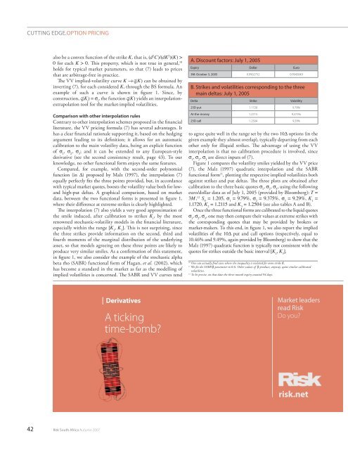The SABR and VV curves tend 42 risk South Africa Autumn 2007 �� A. discount factors: July 1, 2005 expiry dollar euro 3M: october 3, 2005 0.9902752 0.9945049 B. Strikes and volatilities corresponding to the three main deltas: July 1, 2005 delta Strike Volatility 25d put 1.1720 9.79% At-the-money 1.2115 9.375% 25d call 1.2504 9.29% to agree quite well in the range set by the two 10D options (in the given example they almost overlap), typically departing from each other only for illiquid strikes. The advantage of using the VV interpolation is that no calibration procedure is involved, since s 1 , s 2 , s 3 are direct inputs of (7). Figure 1 compares the volatility smiles yielded by the VV price (7), the Malz (1997) quadratic interpolation and the SABR functional form 11 , plotting the respective implied volatilities both against strikes and put deltas. The three plots are obtained after calibration to the three basic quotes s 1 , s 2 , s 3 , using the following euro/dollar data as of July 1, 2005 (provided by Bloomberg): T = 3M, 12 S 0 = 1.205, s 1 = 9.79%, s 2 = 9.375%, s 3 = 9.29%, K 1 = 1.1720, K 2 = 1.2115 and K 3 = 1.2504 (see also tables A and B). Once the three functional forms are calibrated to the liquid quotes s 1 , s 2 , s 3 , one may then compare their values at extreme strikes with the corresponding quotes that may be provided by brokers or market-makers. To this end, in figure 1, we also report the implied volatilities of the 10D put and call options (respectively, equal to 10.46% and 9.49%, again provided by Bloomberg) to show that the Malz (1997) quadratic function is typically not consistent with the quotes for strikes outside the basic interval [K 1 , K 3 ]. 10 One can actually find cases where the inequality is violated for some strike K. 11 We fix the SABR b parameter to 0.6. Other values of b produce, anyway, quite similar calibrated volatilities. 12 To be precise, on that date the three-month expiry counted 94 days. �� Untitled-1 1 5/1/07 12:42:24
Data source: Bloomberg 2 Euro/dollar implied volatilities and their approximations plotted against strikes and put deltas (in absolute value) Implied volatility 0.135 0.130 0.125 0.120 0.115 0.110 0.105 0.100 0.095 Two consistency results for the VV price We now state two important consistency results that hold for the option price (7) and that give further support to the VV procedure. The first result is as follows. One may wonder what happens if we apply the VV curve construction method when starting from three other strikes whose associated prices coincide with those coming from (7). Clearly, for the procedure to be robust, we would want the two curves to exactly coincide. This is indeed the case. In fact, consider a new set of strikes H := {H 1 , H 2 , H 3 }, for which we set: ( ) = ( ) H K i i C H C H 3 ∑ j = 1 BS C H x H ⎡ MKT i j i ⎣ C K j C = ( ) + ( ) ( ) − Vanna-volga smile First-order approximation Second-order approximation 0.090 1.05 1.10 1.15 1.20 1.25 1.30 1.35 Strike BS ( K j ) where the superscripts H and K highlight the set of strikes the pricing procedure is based on, and weights x j are obtained from K with (6). For a generic strike K, denoting by x i (K; H) the weights for K that are derived starting from the set H, the option price associated to H is defined, analogously to (7), by: ( ) = ( 3 ) + ∑ j = 1 ( ) ( ) − ( j ) H BS H BS C K C K x j K; H ⎡ ⎣ C H j C H where the second term in the sum is now not necessarily zero since H 2 is, in general, different from K 2 . The following proposition states the desired consistency result. n Proposition 2. The call prices based on H coincide with those based on K, namely, for each strike K: ⎤ ⎦ ⎤ ⎦ (8) H K C ( K ) = C ( K ) (9) A second consistency result that can be proven for the option price (7) concerns the pricing of European-style derivatives and their static replication. To this end, assume that h(x) is a real function that is defined for x ∈ [0, ∞), is well behaved at infinity and is twice differentiable. Given the simple claim with payout h(S T ) at time T, we denote by V its price at time zero, when taking into account the whole smile of the underlying at time T. By Carr & Madan (1998), we have: Implied volatility 0.135 0.130 0.125 0.120 0.115 0.110 0.105 0.100 0.095 0.090 0 0.1 0.2 0.3 0.4 0.5 0.6 0.7 0.8 0.9 1.0 d f −r T − r T +∞ = ( ) + 0 ′ ( ) + ∫ ′′ ( ) ( ) 0 V e h 0 S e h 0 h K C K dK The same reasoning adopted above (see ‘The VV method: the replicating portfolio’) with regard to the local hedge of the call with strike K can also be applied to the general payout h(S T ). We can thus construct a portfolio of European-style calls with maturity T and strikes K 1 , K 2 and K 3 , such that the portfolio has the same vega, ∂Vega/∂Vol and ∂Vega/∂Spot as the given derivative. Denoting by V BS the claim price under the BS model, this is achieved by finding the corresponding portfolio weights x h 1 , xh and xh, which are always unique (see Proposition 1). We can 2 3 then define a new (smile-consistent) price for our derivative as: 3 Put delta = + ∑ ( ) − ( i ) i= 1 BS h V V x ⎡ MKT BS i ⎣ C Ki C K ⎤ ⎦ (10) which is the obvious generalisation of (7). Our second consistency result is stated in the following. n Proposition 3. The claim price that is consistent with the option prices (7) is equal to the claim price that is obtained by adjusting its BS price by the cost difference of the hedging portfolio when using market prices C MKT (K i ) instead of the constant-volatility prices C BS (K i ). In formulas: V = V Vanna-volga smile First-order approximation Second-order approximation Therefore, if we calculate the hedging portfolio for the claim under flat volatility and add to the BS claim price the cost difference of the hedging portfolio (market price minus constantvolatility price), obtaining V _ , we exactly retrieve the claim price V as obtained through the risk-neutral density implied by the call option prices that are consistent with the market smile. 13 As an example of a possible application of this result, Castagna & Mercurio (2005) consider the specific case of a quanto option, showing that its pricing can be achieved by using the three basic options only, and not the virtually infinite range that is necessary when using static replication arguments. An approximation for implied volatilities The specific expression of the VV option price, combined with the analytical formula (6) for the weights, allows for the derivation 13 Different but equivalent expressions for such a density can be found in Castagna & Mercurio (2005) and Beneder & Baker (2005). www.risksouthafrica.com 43
Page 1 and 2: The vanna-volga method for implied
Page 3: Data source: Bloomberg 1 Implied vo

The vanna-volga method for implied volatilities (PDF - Risk.net

You also want an ePaper? Increase the reach of your titles

Delete template?

Save as template?