The vanna-volga method for implied volatilities (PDF - Risk.net

The vanna-volga method
for implied volatilities
The vanna-volga method is a popular approach for
constructing implied-volatility curves in the options
market. In this article, Antonio Castagna and Fabio
Mercurio give it both theoretical and practical
support by showing its tractability and robustness
The vanna-volga
(VV) method is an
empirical procedure
that can be used to infer an implied-volatility smile from three
available quotes for a given maturity. 1 It is based on the construction
of locally replicating portfolios whose associated hedging costs are
added to corresponding Black-Scholes (BS) prices to produce
smile-consistent values. Besides being intuitive and easy to
implement, this procedure has a clear financial interpretation,
which further supports its use in practice.
The VV method is commonly used in foreign-exchange options
markets, where three main volatility quotes are typically available
for a given market maturity: the delta-neutral straddle, referred to
as at-the-money (ATM); the risk reversal for 25D call and put; and
the (vega-weighted) butterfly with 25D wings. 2 The application of
VV allows us to derive implied volatilities for any option’s delta,
in particular for those outside the basic range set by the 25D put
and call quotes.
In the financial literature, the VV approach was introduced by
Lipton & McGhee (2002), who compare different approaches to
the pricing of double-no-touch options, and by Wystup (2003),
who describes its application to the valuation of one-touch options.
However, their analyses are rather informal and mostly based on
numerical examples. In this article, instead, we will review the VV
procedure in more detail and derive some important results
concerning the tractability of the method and its robustness.
We start by describing the replication argument on which the
VV procedure is based and derive closed-form formulas for the
weights in the hedging portfolio to render the smile construction
more explicit. We then show that the VV price functional satisfies
typical no-arbitrage conditions and test the robustness of the
resulting smile by showing that: changing the three initial pairs of
strike and volatility consistently eventually produces the same
implied-volatility curve; and the VV method, if re-adapted to price
European-style claims, is consistent with static-replication
arguments. Finally, we derive first- and second-order approximations
for the implied volatilities induced by the VV option price.
Since the VV method provides an efficient tool for interpolating
or extrapolating implied volatilities, we also compare it with other
popular functional forms, like that of Malz (1997) and that of
Hagan, et al. (2002).
All the proofs of the propositions in this article are omitted
for brevity. However, they can be found in Castagna & Mercurio
(2005).
The VV method: the replicating portfolio
We consider a foreign-exchange option market where, for a given
maturity T, three basic options are quoted: the 25D put, the ATM
and the 25D call. We denote the corresponding strikes by K i , i = 1,
2, 3, K 1 < K 2 < K 3 , and set K := {K 1 , K 2 , K 3 }. 3 The market-implied
volatility associated with K 1 is denoted by s i , i = 1, 2, 3.
The VV method serves the purpose of defining an impliedvolatility
smile that is consistent with the basic volatilities s i . The
rationale behind it stems from a replication argument in a flat-smile
world where the constant level of implied volatility varies
stochastically over time. This argument is presented hereafter, where,
for simplicity, we consider the same type of options, namely calls.
It is well known that, in the BS model, the payout of a Europeanstyle
call with maturity T and strike K can be replicated by a dynamic
D-hedging strategy, whose value (including the bank account part)
matches, at every time t, the option price C BS (t; K) given by:
BS
( ) =
C t; K S e
−Ke
t
d
−r
t
cutting edge. option pricing
f
−r t
⎛ ln
Φ ⎜
⎝
⎜
St
K
d f 1 2
( 2 )
+ r − r +
s t
( )
⎛ St
d f
+ − −
⎞
K r r s t
Φ ⎜
⎟
⎝
⎜
s t
⎠
⎟
ln 1 2
2
s t ⎞
⎟
⎠
⎟
where S t denotes the exchange rate at time t, t := T – t, r d and r f
denote, respectively, the domestic and foreign risk-free rates, and
s is the constant BS implied volatility. 4 In real financial markets,
however, volatility is stochastic and traders hedge the associated
risk by constructing portfolios that are vega-neutral in a BS (flatsmile)
world.
1 The terms vanna and volga are commonly used by practitioners to denote the partial derivatives
∂Vega/∂Spot and ∂Vega/∂Vol of an option’s vega with respect to the underlying asset and its volatility,
respectively. The reason for naming the procedure this way is made clear below.
2 The ‘%’ sign after the level of the D is omitted, in accordance with market jargon. Therefore, a 25D call is a
call whose delta is 0.25. Analogously, a 25D put is one whose delta is –0.25.
3 For the exact definition of strikes K1 , K 2 and K 3 , we refer to Bisesti, Castagna & Mercurio (2005), where a
thorough description of the main quotes in a foreign-exchange option market is also provided.
4 The option price when the underlying asset is an exchange rate was in fact derived by Garman &
Kohlhagen (1983). Since their formula follows from the BS assumption, we prefer to state we are using the
BS model, also because the VV method can, in principle, be applied to other underlyings.
(1)
www.risksouthafrica.com 39

cutting edge. option pricing
Maintaining the assumption of flat but stochastic implied
volatilities, the presence of three basic options in the market makes
it possible to build a portfolio that zeroes out partial derivatives up
to the second order. In fact, denoting respectively by D and x the
t i
units of the underlying asset and options with strikes K held at
i
BS BS time t and setting C (t) = C (t; Ki ), under diffusion dynamics for
i
both S and s = s , we have by Itô’s lemma:
t t
dC BS t; K
40 risk South Africa Autumn 2007
( ) − ∆t dSt − ∑ xidC i
( )
= ∂C BS ⎡ t; K
⎢
⎣⎢
∂t
( )
+ ∂C BS ⎡ t; K
⎢
⎣⎢
∂S
+ 1 ⎡
⎢
2 ⎣⎢
+ 1 ⎡
⎢
2 ⎣⎢
( )
+ ∂C BS ⎡ t; K
⎢
⎣⎢
∂σ
⎡
⎢
⎣⎢
( )
∂S 2
∂ 2 C BS t; K
( )
∂σ 2
∂ 2 C BS t; K
( )
+ ∂2 C BS t; K
∂S∂σ
3
∑
− x i
i=1
3
∑
3
i=1
− ∆ t − x i
3
∑
i=1
− x i
i=1
3
∑
− x i
i=1
3
∑
− x i
i=1
3
∑
− x i
i=1
( )
BS
∂Ci t
∂t
( )
BS t
BS
∂Ci t
∂S
( )
BS
∂Ci t
∂σ
⎤
⎥ dt
⎦⎥
( )
⎤
⎥
⎦⎥
( )
∂ 2 BS
Ci t
∂S 2
( )
∂ 2 BS
Ci t
∂σ 2
( )
∂ 2 BS
Ci t
∂S∂σ
⎤
⎥
⎦⎥
dσ t
⎤
⎥
⎦⎥
⎤
⎥
⎦⎥
dS t
( ) 2
dS t
( ) 2
dσ t
⎤
⎥ dSt dσ t
⎦⎥
Choosing D t and x i so as to zero out the coefficients of dS t , ds t ,
(ds t ) 2 and dS t ds t , 5 the portfolio comprises a long position in the
call with strike K, and short positions in x i calls with strike K i and
short the amount D t of the underlying, and is locally risk-free at
time t, in that no stochastic terms are involved in its differential 6 :
dC BS t; K
= r d C BS ⎡
⎢ t; K
⎣
( ) − ∆t dSt − ∑ xidC i
3
i=1
( ) − ∆t St − ∑ xiC i
3
i=1
( )
BS t
( )
BS t
⎤
⎥
⎦
dt
Therefore, when volatility is stochastic and options are valued
with the BS formula, we can still have a (locally) perfect hedge,
provided that we hold suitable amounts of three more options to
rule out the model risk. (The hedging strategy is irrespective of
the true asset and volatility dynamics, under the assumption of
no jumps.)
n Remark 1. The validity of the previous replication argument
may be questioned because no stochastic-volatility model can
produce implied volatilities that are flat and stochastic at the same
time. The simultaneous presence of these features – though
inconsistent from a theoretical point of view – can, however, be
justified on empirical grounds. In fact, the practical advantages of
the BS paradigm are so clear that many foreign-exchange option
traders run their books by revaluing and hedging according to a
BS flat-smile model, with the ATM volatility being continuously
updated to the actual market level. 7
The first step in the VV procedure is the construction of the
above hedging portfolio, whose weights x i are explicitly calculated
in the following section.
(2)
(3)
Calculating the VV weights
We assume hereafter that the constant BS volatility is the ATM
one, thus setting s = s 2 (= s ATM ). We also assume that t = 0,
dropping accordingly the argument t in the call prices. From (2),
we see that the weights x 1 = x 1 (K), x 2 = x 2 (K) and x 3 = x 3 (K), for
which the resulting portfolio of European-style calls with
maturity T and strikes K 1 , K 2 and K 3 has the same vega, ∂Vega/
∂Vol and ∂Vega/∂Spot as the call with strike K, 8 can be found by
solving the following system:
∂
( ) = ( )
∂
∂
C
K ∑ x K
∂
C
i
s s
2
∂ C
∂s
2
BS
BS
2
∂ C
∂ ∂
BS
3
i=
1
3
( ) = ∑
i=
1
s S0 i=
1
BS
C
K xi
( K ) ∂
∂s
3
BS
( K )
i
( K )
∂ C
( K ) = ∑ xi ( K )
∂ ∂S
K
s
2
2
2
BS
0
i
( )
Denoting by V(K) the vega of a European-style option with
maturity T and strike K:
BS
∂C
V ( K ) =
∂σ K
( ) = S 0 e− r f T T ϕ d1 K
2
( σ )T
d1 ( K ) = ln S0 K + r d − r f + 1
2
σ T
i
( ( ) )
where j(x) = Φ′(x) is the normal density function, and calculating
the second-order derivatives:
2
BS
( )
∂ C
2
∂
K
( K ) = d1 K d2 K
2
∂ C
( ) = −
∂ ∂S
K
s
V
s
BS V ( K )
d2 ( K )
s S s T
0
( ) = ( ) −
d K d K s T
2 1
we can prove the following.
0
( ) ( )
n Proposition 1. The system (4) admits a unique solution, which
is given by:
x K
1
x K
2
( ) =
( ) =
( ) =
x K
3
( )
( )
V K
V K
1
( )
( )
V K
V K
2
( )
( )
V K
V K
3
K2
K
K3
K
K2
K1
K3
K1
ln ln
ln ln
ln ln
K
K1
K2
K1
ln ln
ln ln
K3
K
K3
K2
K
K1
K
K2
K3
K1
K3
K2
ln ln
In particular, if K = K j then x i (K) = 1 for i = j and zero
otherwise.
The VV option price
We can now proceed to the definition of an option price that is
consistent with the market prices of the basic options.
The above replication argument shows that a portfolio
5 The coefficient of (dSt ) 2 will be zeroed accordingly, due to the relation linking an option’s gamma and
vega in the BS world.
6 We also use the BS partial differential equation.
7 ‘Continuously’ typically means a daily or slightly more frequent update.
8 This explains the name assigned to the smile-construction procedure, given the meaning of the terms
vanna and volga.
(4)
(5)
(6)

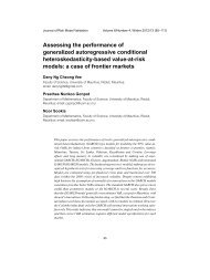
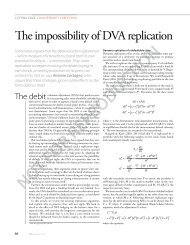
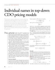
Data source: Bloomberg
1 Implied volatilities plotted against strikes and put deltas (in absolute value), calibrated to the three basic euro/
dollar quotes and compared with the 10D (put and call) volatilities
Implied volatility
0.125
0.120
0.115
0.110
0.105
0.100
0.095
comprising x i (K) units of the option with strike K i (and D 0 units
of the underlying asset) gives a local perfect hedge in a BS world.
The hedging strategy, however, has to be implemented at
prevailing market prices, which generates an extra cost with
respect to the BS value of the options portfolio. Such a cost has to
be added to the BS price (1), with t = 0, to produce an arbitragefree
price that is consistent with the quoted option prices C MKT (K 1 ),
C MKT (K 2 ) and C MKT (K 3 ).
In fact, in case of a short maturity – that is, for a small T – (3)
can be approximated as:
so that setting:
we have:
( ST − K ) + − C BS ( K ) − ∆ 0 [ ST − S0 ]
3
( ) + − C BS ( Ki )
−∑ x ⎡
i ST − Ki ⎣
i=1
≈ r d C BS ⎡
⎢ K
⎣
⎤
⎦
( ) − ∆ 0S0 − xiC BS 3
∑
i=1
Ki 3
( )
⎤
⎥
⎦
T
( ) = ( ) + ∑ ( ) ( ) − ( i )
i=
1
BS
C K C K x K ⎡ MKT
BS
i ⎣
C Ki C K
( ST − K ) + ≈ C ( K ) + ∆ 0 [ ST − S0 ]
3
( ) + − C MKT ( Ki )
+ ∑ x ⎡
i ST − Ki ⎣
i=1
+ r d ⎡
⎢C
K
⎣
Euro/dollar quotes
10∆ (put and call) volatilities
0.090
1.05 1.10 1.15 1.20 1.25 1.30 1.35
Strike
( ) − ∆ 0S0 − xiC MKT 3
∑
i=1
Ki ⎤
⎦
( )
Vanna-volga
Malz
SABR
⎤
⎥
⎦
T
Therefore, when actual market prices are considered, the option
payout (S T – K) + can still be replicated by buying D 0 units of the
underlying asset and x i options with strike K i (investing the
resulting cash at rate r d ), provided one starts from the initial
endowment C(K).
The quantity C(K) in (7) is thus defined as the VV option’s
premium, implicitly assuming that the replication error is also
negligible for longer maturities. Such a premium equals the BS
price C BS (K) plus the cost difference of the hedging portfolio
induced by the market-implied volatilities with respect to the
constant volatility s. Since we set s = s 2 , the market volatility for
⎤
⎦
(7)
Implied volatility
0.125
0.120
0.115
0.110
0.105
0.100
0.095
0.090
0 0.1 0.2 0.3 0.4 0.5 0.6 0.7 0.8 0.9 1.0
strike K 2 , (7) can be simplified to:
( ) = ( ) + ( ) ( ) − ( )
C K
BS
C K x1 K ⎡ MKT
⎣
C K1 BS
C K1
⎤
⎦
+ x3 ( K ) ⎡ MKT BS
⎣
C ( K3 ) − C ( K3
) ⎤
⎦
n Remark 2. Expressing the system (4) in the form b = Ax and
setting c = (c 1 , c 2 , c 3 )′, where c i := C MKT (K i ) – C BS (K i ), and y = (y 1 ,
y 2 , y 3 )′ := (A′) –1 c, we can also write:
C K C K y C
BS
∂
( ) = ( ) + 1
∂s
2
∂ C
+ y2
∂s
BS
2
( ) +
K y
3
2
BS
BS
( K )
∂ C
S K
∂s∂ 0
( )
The difference between the VV and BS prices can thus be
interpreted as the sum of the option’s vega, ∂Vega/∂Vol and
∂Vega/∂Spot, weighted by their respective hedging cost y. 9 Besides
being quite intuitive, this representation also has the advantage
that the weights y are independent of the strike K and, as such,
can be calculated once for all. However, we prefer to stick to the
definition (7), since it allows an easier derivation of our
approximations below.
The VV option price has several interesting features that we
analyse in the following.
When K = K j , C(K j ) = C MKT (K j ), since x i (K) = 1 for i = j and
zero otherwise. Therefore, (7) defines a rule for either interpolating
or extrapolating prices from the three option quotes C MKT (K 1 ),
C MKT (K 2 ) and C MKT (K 3 ).
The option price C(K), as a function of the strike K, is twice
differentiable and satisfies the following (no-arbitrage) conditions:
lim C K S e and lim C K
lim
Euro/dollar quotes
10∆ (put and call) volatilities
Put delta
Vanna-volga
Malz
SABR
+
K →0
( ) = 0
f
−r
T
K →+∞ ( ) = 0
d
dC
−r
T
+
K →0
dK ( K ) = − e dC
K →+∞ K dK ( K ) =
and lim 0
These properties, which are trivially satisfied by C BS (K), follow
from the fact that, for each i, both x i (K) and dx i (K)/dK go to zero
for K → 0 + or K → +∞.
To avoid arbitrage opportunities, the option price C(K) should
9 The authors thank one of the referees for suggesting this alternative formulation.
www.risksouthafrica.com 41

cutting edge.option pricing
also be a convex function of the strike K, that is, (d 2 C)/(dK 2 )(K) >
0 for each K > 0. This property, which is not true in general, 10
holds for typical market parameters, so that (7) leads to prices
that are arbitrage-free in practice.
The VV implied-volatility curve K → ς(K) can be obtained by
inverting (7), for each considered K, through the BS formula. An
example of such a curve is shown in figure 1. Since, by
construction, ς(K i ) = s i , the function ς(K) yields an interpolationextrapolation
tool for the market-implied volatilities.
Comparison with other interpolation rules
Contrary to other interpolation schemes proposed in the financial
literature, the VV pricing formula (7) has several advantages. It
has a clear financial rationale supporting it, based on the hedging
argument leading to its definition; it allows for an automatic
calibration to the main volatility data, being an explicit function
of s 1 , s 2 , s 3 ; and it can be extended to any European-style
derivative (see the second consistency result, page 43). To our
knowledge, no other functional form enjoys the same features.
Compared, for example, with the second-order polynomial
function (in D) proposed by Malz (1997), the interpolation (7)
equally perfectly fits the three points provided, but, in accordance
with typical market quotes, boosts the volatility value both for low-
and high-put deltas. A graphical comparison, based on market
data, between the two functional forms is presented in figure 1,
where their difference at extreme strikes is clearly highlighted.
The interpolation (7) also yields a very good approximation of
the smile induced, after calibration to strikes K i , by the most
renowned stochastic-volatility models in the financial literature,
especially within the range [K 1 , K 3 ]. This is not surprising, since
the three strikes provide information on the second, third and
fourth moments of the marginal distribution of the underlying
asset, so that models agreeing on these three points are likely to
produce very similar smiles. As a confirmation of this statement,
in figure 1, we also consider the example of the stochastic alpha
beta rho (SABR) functional form of Hagan, et al. (2002), which
has become a standard in the market as far as the modelling of
implied volatilities is concerned. The SABR and VV curves tend
42 risk South Africa Autumn 2007
������������
���������
����������
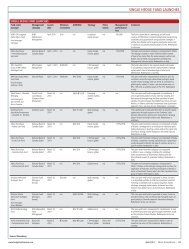
A. discount factors: July 1, 2005
expiry dollar euro
3M: october 3, 2005 0.9902752 0.9945049
B. Strikes and volatilities corresponding to the three
main deltas: July 1, 2005
delta Strike Volatility
25d put 1.1720 9.79%
At-the-money 1.2115 9.375%
25d call 1.2504 9.29%
to agree quite well in the range set by the two 10D options (in the
given example they almost overlap), typically departing from each
other only for illiquid strikes. The advantage of using the VV
interpolation is that no calibration procedure is involved, since
s 1 , s 2 , s 3 are direct inputs of (7).
Figure 1 compares the volatility smiles yielded by the VV price
(7), the Malz (1997) quadratic interpolation and the SABR
functional form 11 , plotting the respective implied volatilities both
against strikes and put deltas. The three plots are obtained after
calibration to the three basic quotes s 1 , s 2 , s 3 , using the following
euro/dollar data as of July 1, 2005 (provided by Bloomberg): T =
3M, 12 S 0 = 1.205, s 1 = 9.79%, s 2 = 9.375%, s 3 = 9.29%, K 1 =
1.1720, K 2 = 1.2115 and K 3 = 1.2504 (see also tables A and B).
Once the three functional forms are calibrated to the liquid quotes
s 1 , s 2 , s 3 , one may then compare their values at extreme strikes with
the corresponding quotes that may be provided by brokers or
market-makers. To this end, in figure 1, we also report the implied
volatilities of the 10D put and call options (respectively, equal to
10.46% and 9.49%, again provided by Bloomberg) to show that the
Malz (1997) quadratic function is typically not consistent with the
quotes for strikes outside the basic interval [K 1 , K 3 ].
10 One can actually find cases where the inequality is violated for some strike K.
11 We fix the SABR b parameter to 0.6. Other values of b produce, anyway, quite similar calibrated
volatilities.
12 To be precise, on that date the three-month expiry counted 94 days.
���������������
���������
�������
��������
Untitled-1 1 5/1/07 12:42:24

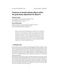
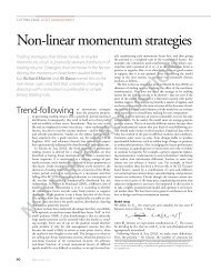
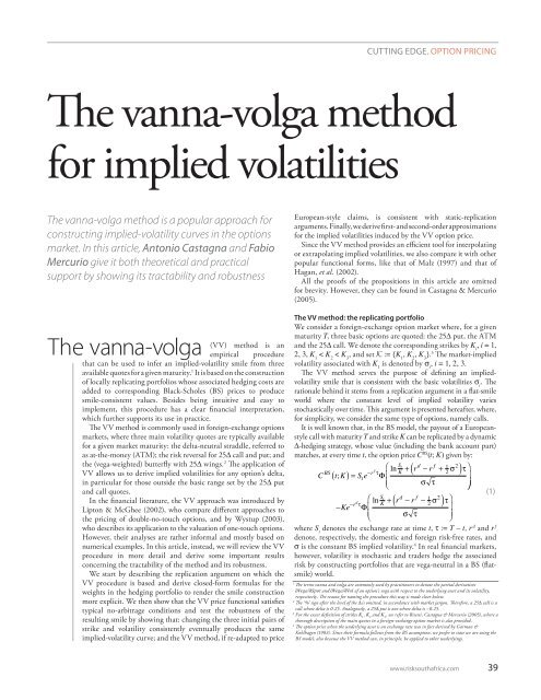
Data source: Bloomberg
2 Euro/dollar implied volatilities and their approximations plotted against strikes and put deltas (in absolute value)
Implied volatility
0.135
0.130
0.125
0.120
0.115
0.110
0.105
0.100
0.095
Two consistency results for the VV price
We now state two important consistency results that hold
for the option price (7) and that give further support to the
VV procedure.
The first result is as follows. One may wonder what happens if
we apply the VV curve construction method when starting from
three other strikes whose associated prices coincide with those
coming from (7). Clearly, for the procedure to be robust, we
would want the two curves to exactly coincide. This is indeed
the case.
In fact, consider a new set of strikes H := {H 1 , H 2 , H 3 }, for
which we set:
( ) = ( )
H K
i i
C H C H
3
∑
j = 1
BS
C H x H ⎡ MKT
i j i ⎣
C K j C
= ( ) + ( ) ( ) −
Vanna-volga smile
First-order approximation
Second-order approximation
0.090
1.05 1.10 1.15 1.20 1.25 1.30 1.35
Strike
BS
( K j )
where the superscripts H and K highlight the set of strikes the
pricing procedure is based on, and weights x j are obtained from K
with (6). For a generic strike K, denoting by x i (K; H) the weights
for K that are derived starting from the set H, the option price
associated to H is defined, analogously to (7), by:
( ) = (
3
) + ∑
j = 1
( ) ( ) − ( j )
H BS
H
BS
C K C K x j K; H ⎡
⎣
C H j C H
where the second term in the sum is now not necessarily zero
since H 2 is, in general, different from K 2 . The following proposition
states the desired consistency result.
n Proposition 2. The call prices based on H coincide with those
based on K, namely, for each strike K:
⎤
⎦
⎤
⎦
(8)
H K
C ( K ) = C ( K ) (9)
A second consistency result that can be proven for the option
price (7) concerns the pricing of European-style derivatives and
their static replication. To this end, assume that h(x) is a real
function that is defined for x ∈ [0, ∞), is well behaved at infinity
and is twice differentiable. Given the simple claim with payout
h(S T ) at time T, we denote by V its price at time zero, when taking
into account the whole smile of the underlying at time T. By Carr
& Madan (1998), we have:
Implied volatility
0.135
0.130
0.125
0.120
0.115
0.110
0.105
0.100
0.095
0.090
0 0.1 0.2 0.3 0.4 0.5 0.6 0.7 0.8 0.9 1.0
d f
−r T − r T
+∞
= ( ) + 0 ′ ( ) + ∫ ′′ ( ) ( )
0
V e h 0 S e h 0 h K C K dK
The same reasoning adopted above (see ‘The VV method: the
replicating portfolio’) with regard to the local hedge of the call
with strike K can also be applied to the general payout h(S T ). We
can thus construct a portfolio of European-style calls with
maturity T and strikes K 1 , K 2 and K 3 , such that the portfolio has
the same vega, ∂Vega/∂Vol and ∂Vega/∂Spot as the given
derivative. Denoting by V BS the claim price under the BS model,
this is achieved by finding the corresponding portfolio weights x h
1 ,
xh and xh,
which are always unique (see Proposition 1). We can
2 3
then define a new (smile-consistent) price for our derivative as:
3
Put delta
= + ∑ ( ) − ( i )
i=
1
BS h
V V x ⎡ MKT
BS
i ⎣
C Ki C K
⎤
⎦
(10)
which is the obvious generalisation of (7). Our second consistency
result is stated in the following.
n Proposition 3. The claim price that is consistent with the
option prices (7) is equal to the claim price that is obtained by
adjusting its BS price by the cost difference of the hedging
portfolio when using market prices C MKT (K i ) instead of the
constant-volatility prices C BS (K i ). In formulas:
V = V
Vanna-volga smile
First-order approximation
Second-order approximation
Therefore, if we calculate the hedging portfolio for the claim
under flat volatility and add to the BS claim price the cost
difference of the hedging portfolio (market price minus constantvolatility
price), obtaining V _ , we exactly retrieve the claim price V
as obtained through the risk-neutral density implied by the call
option prices that are consistent with the market smile. 13
As an example of a possible application of this result, Castagna
& Mercurio (2005) consider the specific case of a quanto option,
showing that its pricing can be achieved by using the three basic
options only, and not the virtually infinite range that is necessary
when using static replication arguments.
An approximation for implied volatilities
The specific expression of the VV option price, combined with
the analytical formula (6) for the weights, allows for the derivation
13 Different but equivalent expressions for such a density can be found in Castagna & Mercurio (2005)
and Beneder & Baker (2005).
www.risksouthafrica.com 43

cutting edge. option pricing
of a straightforward approximation for the VV implied volatility
ς(K), by expanding both members of (7) at first order in s = s 2 .
We obtain:
ς( K ) ≈ ς1 K
44 risk South Africa Autumn 2007
+ ln K
ln K1 K 3
K
ln K 2 ln K1 K 3
K 2
( ) := ln K 2
σ 2 +
K ln K 3
K
ln K 2 ln K1 K 3
K1 K ln ln K1 K
K 2
ln K 3 ln K1 K 3
K 2
σ 1
σ 3
(11)
The implied volatility ς(K) can thus be approximated by a linear
combination of the basic volatilities s , with coefficients that add
i
up to one (as tedious but straightforward algebra shows). It is also
easily seen that the approximation is a quadratic function of lnK,
so that one can resort to a simple parabolic interpolation when log
co-ordinates are used.
A graphical representation of the accuracy of the approximation
(11) is presented in figure 2, where we use the same euro/dollar
data as for figure 1. The approximation (11) is extremely accurate
inside the interval [K , K ]. The wings, however, tend to be
1 3
overvalued. In fact, being the quadratic functional form in the
log-strike, the no-arbitrage conditions derived by Lee (2004) for
the asymptotic value of implied volatilities are violated. This
drawback is addressed by a second, more precise, approximation,
which is asymptotically constant at extreme strikes, and is obtained
by expanding both members of (7) at second order in s = s : 2
ς( K ) ≈ ς 2 ( K ) := σ 2
where:
+ −σ 2 + σ 2
2 + d1 K
D1 ( K ) := ς1 ( K ) − σ 2
D 2 K
+ ln K
( ) := ln K 2
ln K1 K
K 2
ln K 3 ln K1 K 3
K 2
( ) ( 2σ 2 D1 ( K ) + D2 ( K ) )
( )
( )d 2 K
d1 ( K )d 2 K
K ln K 3
K
ln K 2 ln K1 K 3
K1 d1 ( K1 )d 2 ( K1 ) ( σ1 − σ 2 ) 2
d1 ( K 3 )d 2 ( K 3 ) ( σ 3 − σ 2 ) 2
(12)
As we can see from figure 2, the approximation (12) is also
extremely accurate in the wings, even for extreme values of put
deltas. Its only drawback is that it may not be defined, due to the
presence of a square-root term. The radicand, however, is positive
in most practical applications.
References
Beneder R and G Baker, 2005
Pricing multi-currency options
with smile
Internal report, ABN Amro
Bisesti L, A Castagna and F Mercurio,
2005
Consistent pricing and hedging of an
FX options book
Kyoto Economic Review 74(1),
pages 65–83
Carr P and D Madan, 1998
Towards a theory of volatility trading
Volatility, R Jarrow (ed.), Risk Books,
pages 417–427
Castagna A and F Mercurio, 2005
Consistent pricing of FX options
Internal report, Banca IMI,
available at www.fabiomercurio.it/
consistentfxsmile2b.pdf
Garman B and S Kohlhagen, 1983
Foreign currency option values
Journal of International Money and
Finance 2, pages 231–237
Conclusions
We have described the VV approach, an empirical procedure to
construct implied volatility curves in the foreign exchange
market. We have seen that the procedure leads to a smileconsistent
pricing formula for any European-style contingent
claim. We have also compared the VV option prices with those
coming from other functional forms known in the financial
literature. We have then shown consistency results and proposed
efficient approximations for the VV implied volatilities.
The VV smile-construction procedure and the related pricing
formula are rather general. In fact, even though they have been
developed for foreign exchange options, they can be applied in
any market where at least three reliable volatility quotes are
available for a given maturity. The application also seems quite
promising in other markets, where European-style exotic payouts
are more common than in the foreign exchange market. Another
possibility is the interest rate market, where CMS convexity
adjustments can be calculated by combining the VV price
functional with the replication argument in Mercurio &
Pallavicini (2006).
A last, unsolved issue concerns the valuation of pathdependent
exotic options by means of a generalisation of the
empirical procedure that we have illustrated in this article. This
is, in general, a quite complex issue to deal with, considering
also that the quoted implied volatilities only contain
information on marginal densities, which is of course not
sufficient for valuing path-dependent derivatives. For exotic
claims, ad hoc procedures are usually used. For instance, barrier
option prices can be obtained by weighing the cost difference
of the ‘replicating’ strategy by the (risk-neutral) probability of
not crossing the barrier before maturity (see Lipton & McGhee
(2002) and Wystup (2003) for a description of the procedure
for one-touch and double-no-touch options, respectively).
However, not only are such adjustments harder to justify
theoretically than those in the plain vanilla case, but, from a
practical point of view, they can even have the opposite sign
with respect to that implied in market prices (when very steep
and convex smiles occur). We leave the analysis of this issue to
future research. n
Antonio castagna is an equity derivatives trader at Banca profilo, Milan. Fabio
Mercurio is head of financial modelling at Banca iMi, Milan. they would like to
thank giulio Sartorelli and three anonymous referees for their comments and
helpful suggestions. email: antonio.castagna@bancaprofilo.it
fabio.mercurio@bancaimi.it
Hagan P, D Kumar, A Lesniewski
and D Woodward, 2002
Managing smile risk
Wilmott, September, pages 84–108
Lee R, 2004
The moment formula for implied
volatility at extreme strikes
Mathematical Finance 14(3),
pages 469–480
Lipton A and W McGhee, 2002
Universal barriers
Risk May, pages 81–85
Malz A, 1997
Estimating the probability distribution
of the future exchange rate from option
prices
Journal of Derivatives, winter,
pages 18–36
Mercurio F and A Pallavicini, 2006
Smiling at convexity
Risk August, pages 64–69
Wystup U, 2003
The market price of one-touch options
in foreign exchange markets
Derivatives Week 12(13), pages 1–4