Leakage-aware energy synchronization for wireless sensor networks

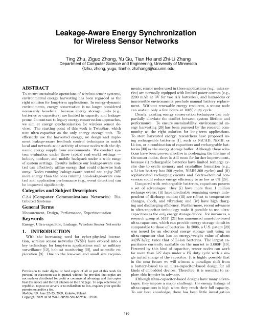
Leakage Power (mW)1098765432122F33F50F100F10 −1 10 0 10 1 10 2 10 3Time (Hour)010 −1 10 0 10 1 10 2 10 3Time (Hour)(a) Small Capacitance (b) Large CapacitanceFigure 4: Leakage Power vs. Timethis big uncertainty would lead to ineffective energy control.Impact of Battery Type: We also conducted a series ofexperiments to investigate the consistency of battery modelsover different battery types. In this study, three differenttypes of the batteries are investigated: Li-ion, NiCADand NiMH. Comparing Figures 2a, 2b, and 2c indicates thatdifferent types of the batteries have different discharge characteristicsand different capacities. In other words, thereis no single battery model that can be applied to differentbattery types. For example, when a sensor node runs underthe 1%-LED workload, remaining energy under 2.7V is 3.8kJ, 10.55 kJ, and 22.16 kJ for Li-ion, NiCAD, and NiMHbatteries, respectively.Figure 2 also shows that the discharge curves for differentbatteries exhibit deep slopes within a certain voltage range,in which a small error in voltage reading would be amplifiedinto a large error in estimating remaining energy. Forexample, as shown in Figure 2b, an 0.1V error would betranslated into a 200% energy difference between 2.4V and2.5V readings.Leakage Power (mW)150120906030650F2000F3000F2.2 Leakage in the Energy StoragesThis section presents our empirical study on the leakageprofile of batteries and ultra-capacitors. We conducted experimentsover a period of 6 weeks, using different typesof batteries and ultra-capacitors. Our empirical study concludesthat (i) ultra-capacitors are a good substitute for batteriesand (ii) energy leakage in ultra-capacitors should notbe overlooked.Leakage Profile Comparison: To simplify the comparisonagainst ultra-capacitors, Li-ion batteries are chosen asrepresentatives of the other batteries. We conducted leakageprofile comparisons between Li-ion batteries and a 2,000Fultra-capacitor over a period of 2 months after they arefully charged. For Li-ion battery, the leakage rate is 8% permonth. The 2,000F ultra-capacitor has a very high leakagerate (43.8%) during the first month, but low leakage rate(5.26%) during the second month. At the end of the secondmonth, the ultra-capacitor still has 1.9V of remainingvoltage. These results indicate that ultra-capacitors haveleakage performance that is comparable to that of batterieswhen voltage is controlled under an appropriate level. However,ultra-capacitors suffer severe energy leakage when it ischarged to the limit.Leakage of Ultra-Capacitors: In this experiment, seventypes of ultra-capacitors are used, ranging from 22F to3000F. After an ultra-capacitor was fully charged, we isolatedit and continuously monitored its remaining voltageover 1000 hours. Figure 4 reveals that (i) the leakage powerreduces over time after the initial charge, and (ii) leakageis more severe for larger ultra-capacitors than for smallerultra-capacitors. For example, at 2.7V, the leakage power ofa 3,000F capacitor is about 17 times of that of a 100F.Leakage Power (mW)1098765432122F33F50F100F0.8 1 1.2 1.4 1.6 1.8 2 2.2 2.4 2.6 2.8Voltage Measured (V)01.8 2 2.2 2.4 2.6 2.8Voltage Measured (V)(a) Small Capacitance (b) Large CapacitanceFigure 5: Leakage Power vs. VoltagesRemaining Energy (J)160140120Leakage Power (mW)150120906030650F2000F3000FWith LeakageWithout Leakage1008060402000 10 20 30 40 50 60 70Time (Hour)Figure 6: Remaining Energy Vs. TimeWe also investigated the correlation between the voltageand leakage of ultra-capacitors. Figure 5 shows that whenthe voltage of ultra-capacitors approaches its limit, the valueof leakage power increases significantly. For example, whenthe voltage of the 100F ultra-capacitor increases to 2.7V, itsleakage power is 8.4 mW, which is equivalent to the powerneeded for powering a Telos node to work under more than13% duty cycle.Lifetime Difference due to Leakage: With the empiricaldata collected, we simulate the lifetime of a node consideringleakage. Figure 6 compares the remaining energy insidethe ideal non-leaking ultra-capacitor and the real ultracapacitorwith leakage. Here we use a fully charged 50Fultra-capacitor, to power a MicaZ node at 1% duty cycle.We can see that ideally, without leakage the MicaZ node’slifetime would be 65 hours, but because of the leakage, theMicaZ node’s lifetime is actually only 49 hours, or 24% lessthan the lifetime we would otherwise expect.3. OVERVIEW OF SYSTEM DESIGNThe empirical study in Section 2 indicates that energyleakage is a critical hurdle that hinders designers exploitingthe benefits of ultra-capacitor over batteries. To address thehurdle, we propose a three-layer design as shown in Figure 7.AdaptationLayerControlLayerHardwareLayerEnvironmentMonitoringDuty CycleControllerEnergyStorageSuggestedDuty CycleEnergyInformationMilitary...SurveillanceLeakageLifetimePredictorHarvestingFigure 7: Overview of System Architecture• The hardware layer uses an energy harvesting circuit (e.g.,solar panel or wind generator) to harvest the environmentalenergy and uses an ultra-capacitor as the only energy storageunit to power sensor nodes. This layer also (i) monitors theremaining energy inside the ultra-capacitor, (ii) samples theenergy harvesting rate from the energy harvesting circuit,and (iii) models the leakage profile of the capacitor. Thesethree pieces of information are then fed into the control layer.321

Working NodeMain Panel & Peripheral CircuitPower Measurement SwitchEnergy Storage (Ultra-capacitor)Smart Power Supply CircuitEnergy FlowCompanion Node (optional)Separate Power SupplyMonitor & Control FlowFigure 8: TwinStar Hardware Architecture• The control layer predicts the lifetime of a node based onthe energy harvesting, leakage, and consumption rates. Thedifference between the predicted lifetime and user-specifiedlifetime is used as the control signal to the duty cycle controller,which suggests a certain percentage of duty cyclechange to the application. The control layer deals with twoconditions: energy oversupply and undersupply. In the caseof oversupply, the controller prevents the ultra-capacitorfrom charging to its limit, hence reducing the energy leakedaway. In the case of undersupply, the controller signals therunning program to reduce the rate of energy consumptionso as to ensure the minimal but critical activities of the sensornode at any time.• In the adaptation layer, a running application changes itsworking schedules according to the suggested energy budget.Adaptation can be archived by changing per-component activitiesin communication and sensing as well as per-flowactivities [15]. We note that designs for the adaption layerare highly diverse. Instead of using a case-by-case approach,we propose a generic adaptation technique by treating dutycycleas first-class resource that can be allocated, scheduledand adjusted in Section 7.4. HARDWARE DESIGN OF TWINSTARTwinStar is an add-on power board that harvests energyfrom environments and uses an ultra-capacitor as the onlyenergy storage to overcome the intrinsic limitations of batteries(e.g., energy uncertainty, limited recharge cycles, lowconversion efficiency, and environment unfriendliness). Thearchitecture of TwinStar is shown in Figure 8. It consistsof (i) the solar panels and peripheral circuit for energy harvesting;(ii) the power measurement switch; (iii) the ultracapacitor-basedenergy storage; and (iv) the smart powersupply circuit with a DC/DC converter for powering theworking node attached to the TwinStar board. The correspondingprinted circuit board is shown in Figure 9. Due tospace constraints, we only explain a few unique features ofthe TwinStar design in the rest of the section.4.1 Smart Power Supply CircuitTo accommodate fluctuating ambient energy, the voltageof a power supply shall be stabilized. We apply a highefficiencyswitch-type DC/DC converter for providing a stablepower supply for the working node. In the battery-basedapproaches, normally a DC/DC converter is powered directlyby a battery, assuming enough energy is left in thebattery [15, 16]. However, it would be problematic forthe ultra-capacitor-based design, especially under extremelylow ambient energy situations due to the zero-energy bootstrapproblem: Initially, the voltage of the ultra-capacitoris around 0 and all the system components do not workincluding the DC/DC converter. When the voltage of theultra-capacitor reaches a threshold level, the converter entersa warming up stage, during which the high-efficiencySmart PowerSupply CircuitConnector forWorking NodePowerMeasurementSwitchMain PanelConnectionIsolation Circuitfor CompanionNodeConnector forCompanionNodeUltra-CapacitorConnectionBoot PanelConnectionFigure 9: TwinStar Platformswitch-type converter needs to excite the external inductorinto oscillations with high transient current (at the level of10mA). If the scavenged energy is not sufficient to supportthe converter to finish this stage, the voltage of the ultracapacitordrops below the threshold level and the converterfails to boot up. Such failure repeats itself, wasting energyharvested from the environment.To address this zero-energy boot-up challenge, a smartcontrol circuit is designed to automatically boot-up and shutdown the DC/DC converter. The basic idea is that duringthe charging state, the DC/DC converter is kept shutdown by the smart control circuit until the ultra-capacitoraccumulates sufficient energy and reaches a voltage muchhigher than the DC/DC converter’s input voltage threshold(1.1V); during the discharging period, the DC/DC converteris turned off when the voltage of the ultra-capacitorapproaches the minimum input voltage (0.7V). In this way,high boot-up current stage and energy waste can be avoided.However, achieving this kind of smart control needs toovercome a hidden challenge: there is no appropriate powersupply for the smart control circuit itself before enabling theDC/DC converter. In our design, we address all the abovechallenges by proposing a novel dual solar panel solution(a small boot solar panel and a big main panel) togetherwith a Schmitt trigger-based control circuit. The design isillustrated in Figure 10.As shown in Figure 10, a small boot solar panel is appliedto power the Schmitt trigger module that is used to controlthe on/off status of the DC/DC converter. The small panelcharges a small capacitor (C1, which is 47µF) and keeps thevoltage of C1 higher than 2.5V so as to power the Schmitttrigger, which is an extremely low power device with powerconsumption less than 10µW. Therefore, even with a lowenvironmental energy supply, the smart control circuit canstill work.The main panel is the one harvesting energy for the ultracapacitor.Note that when the DC/DC converter starts towork, its output also feeds back to power the Schmitt trigger,avoiding shutting down the DC/DC converter when thereis no environmental energy but the ultra-capacitor is stillenergy-rich.Boot-up & Shutdown CircuitD2D1BootPanelMain Panel&PeripheralCircuit47uFC1PowerSchmittTrigger OutUltracapacitorInC2SHDNDC/DCConverterInOut Power3V SensorNodeFigure 10: Boot-up and Shutdown Control Circuit322

4.2 Ultra-Low-Power Measurement SwitchTo enable the control middle layer to accurately predictthe lifetime of the sensor node, the hardware provides powermeasurement capabilities. Keeping in mind that it is importantto make the measurement circuit simple and energyefficient, we used P-channel MOSFET as the switches (K 1and K 2 as shown in Figure 11), which are controlled by thesensor node.Main Panel&PeripheralCircuitCTL1 (MicaZ)K 1R 1K 2CTL2 (MicaZ)ADC4 ADC6I cap(t)UltracapacitorFigure 11: Power Measurement CircuitNormally the switch K 1 is kept on to harvest environmentalenergy. When measuring the energy harvested into theultra-capacitor, K 1 is switched off and K 2 is turned on bythe control signals from the sensor node. In our implementation,we use MicaZ node and its ADC4 and ADC6 pinsextract the voltage across the resister R 1. Since the resistanceof the resistor R 1 is known, the current I cap(t) goesthrough R 1 can be calculated.The power consumption of the P-MOSFET switch is extremelylow, at the level of nW, and thus negligible. A verysmall resister R 1 is used for the voltage formation and usedonly during the measurement moment (at the level of µs),therefore having a negligible effect on the charging efficiencyfor the ultra-capacitor.4.3 External Sensor NodesOur system supports two external sensor nodes: (i) aworking node, (ii) an optional companion node. The workingnode is powered solely by the ultra-capacitor. It periodicallysamples the voltage of the ultra-capacitor. Based onthe sampled value it calculates the remaining energy insidethe ultra-capacitor. It also periodically controls the powermeasurement switch to measure the environmental powerand calculate the harvested energy.In order to analyze the system performance and supporton-line debugging, the TwinStar platform also contains theinterface for attaching an optional companion node (in Figure9). It is powered and functions separately. Isolation isimportant here because this design prevents the companionnode’s interfering with the working node (in Figure 9).The companion node has three capabilities: (i) periodicallysampling the voltage of the ultra-capacitor, (ii) periodicallymeasuring the energy charged into the ultra-capacitor,and (iii) logging data. Since the companion node is poweredby a separate energy source, it does not have energy constraintduring a short experiment period. The informationcaptured in the first two functions can either be written intothe companion node’s flash memory or transmitted via radio,supporting either off-line or on-line analysis and debugging.All the measurements conducted by the companionnode is protected by voltage follower circuits to avoid loadeffects and achieve isolation.We note that the working node can run alone without thecompanion node. It only needs to monitor its energy statusat a low frequency for control purpose. The main purposeof adding the companion node is to accurately monitor oursystem’s performance at a high frequency for evaluation purpose.By using a companion node, the observer affect canbe avoided, otherwise the working node has to monitor andrecord energy status by itself. These operations consume alot of energy that is not part of workload, causing inaccuracyin performance evaluation.4.4 Summary of Hardware DesignThe TwinStar node has a battery-free hardware structureusing a combination of an ultra-capacitor and solar panels.It has several features that match our requirements:• Stability: To the best of our knowledge, it is the firstdesign that considers the zero-energy boot up challenge anduses a dual-panel structure comprising a boot panel and aharvesting panel. The boot panel ensures stable power harvestingunder extremely low ambient energy situations. Theharvesting panel is used as the main charging device for theultra-capacitor. DC/DC converter provides stable output topower the working node.• Visibility: As an experimental platform, the TwinStarnode provides monitoring/debug interfaces for attaching anadditional companion node (as shown in Figure 9), whichcan help us understand the behaviors of the running workingnode and facilitate system debugging and performanceevaluation. The separate power supply for the companionnode ensures accurate characterizing of the energy profile ofthe working node. In the commercial release version, thiscompanion node can be easily removed to reduce cost.5. SYSTEM ENERGY MODELINGSystem modeling is an essential step for effective control.In this section, we introduce three models: the energy harvestingmodel (Section 5.1), the energy consumption model(Section 5.2) and the energy leakage model (Section 5.3).To achieve effective energy synchronization, we need to balancethe interaction among these models into an equilibriumstate.5.1 Energy Harvesting ModelThe energy harvesting model is built online using the measurementswitch discussed in Section 4.2. The total energyE E harvested during the time interval [(k − 1)T, kT] is:∆E E[kT] =Z kT(k−1)TI cap(t) · V cap(t)dt (1)Here V cap(t) is the ultra-capacitor’s voltage at time t.Both I cap(t) and V cap(t) can be measured by the ultra-lowpowermeasurement switch shown in Figure 11. T is calledthe sampling period and k is called the sampling instant.5.2 Energy Consumption ModelThe energy consumption of the sensor node is determinedby three parameters: average active mode current I active,average sleep mode current I sleep and duty cycle D (thepercentage of active time). The energy consumption duringthe time interval [(k − 1)T, kT] can be represented as:∆E C[kT] = V node · (I active · D + I sleep · (1 − D)) · T (2)The average power consumption at the end of time kTcan be represented as follows:P CAV G(kT) = ∆EC[kT] (3)T5.3 Energy Leakage ModelBased on our empirical study in Section 2, we formulatea leakage model to characterize the relationship betweenthe remaining energy in the ultra-capacitor and the leakagepower. To minimize the environmental effect, such as323

Adaptation LayerAdaptive Componentsn thpredictionT targetT targetControl LayerT diffDuty CycleControllerD suggestE cLifetimePredictorT expect2 nd prediction1 st predictionExpected lifetime… .. ….. ….SurplusT expectExpected lifetime DeficitHardware LayerEnergy StorageLeakageHarvestingExpected lifetimeDeficitTime LineFigure 13: Control Layer Design Overviewtemperature, the leakage model is normally obtained off-lineand can be adjusted online after deployment.To conduct off-line modeling, the harvesting circuit is shutdown and the node executes a testing program at a constantduty cycle. At the end of every T seconds, the control layerperiodically monitors the remaining voltage V cap(t) of theultra-capacitor. Therefore, the difference of remaining energy∆E R[kT] during the time interval [(k −1)T, kT] can becalculated as:∆E R[kT] = C `Vcap((k − 1)T) 2 − V 2´cap(kT)2= E R ((k − 1)T) − E R(kT) (4)Without energy harvesting, ∆E R[kT] is the sum of theenergy consumed by the node and energy leaked away duringtime interval [(k − 1)T, kT], namely∆E R[kT] = ∆E C[kT] +Z kT(k−1)TP L(t)dtFor small value of T, the above equation can be simplifiedas:∆E R[kT] = ∆E C[kT] + P L(kT) · T (5)By combining Equations (4) and (5), at the end of anygiven time kT, the leakage power P L can be calculated bythe sensor node as follows:ER((k − 1)T) − ER(kT) − ∆EC[kT]P L(kT) = (6)TThe sensor node builds the leakage model by storing thevalue of P L(kT) and the corresponding E R(kT) value in itsmemory. Figure 12(a) shows the empirical leakage data ofthe leakage model for diverse capacitors. To express themodel mathematically and reduce the storage space for theLeakage Power (mW)Leakage Power (mW)1098765432110987654321400400300 200 100Remaining Energy (J)22F33F50F100F(a) Empirical Leakage Pattern300 200 100Remaining Energy (J)RealModel(b) Leakage Model FittingFigure 12: Leakage Model00Figure 14: Sustainabilitymodel, we use a piecewise linear approximation of the leakagecurve. We define turning points as the points in thecurve with considerable slope change, which are used to decidethe start and end points of line segments. Therefore,the whole leakage model can be represented by a set of linearfunctions, as shown in Eqn.(7).8a 1 · E R + b 1; E R1 ≤ E R < E R2>< a 2 · E R + b 2; E R2 ≤ E R < E R3P L(E R) =(7). ;.>:a n · E R + b n; E Rn ≤ E R ≤ E Rn+1Here E R1 , E R2 ,· · ·, E Rn+1 are the remaining energy valuescorresponding to the turning points of the segments. a 1,a 2,· · ·, a n and b 1, b 2,· · · , b n are the coefficients for eachline segment. Figure 12(b) shows an example for the linesegment-basedmodeling of the leakage power. The squaredots represent the turning points. The model we built accuratelymatches the empirical results.6. CONTROL LAYER DESIGNThe design objective of the control layer is to consumeas much energy as possible while maintaining sustainability.Sustainability T target is defined as the duration a node mustsurvive without ambient energy. T target is a configurable parameter,set by users according to the environment in whichsensors are deployed. For example, in energy-rich environmentssuch as deserts, users can set a smaller T target to consumeenergy aggressively. On the other hand, in energy-poorand unpredictable environments, a larger T target is desiredto ensure the aliveness of sensor nodes. Once T target is chosen,it is used as the set point in the feedback control baseddesign as shown in Figure 13.As shown in Figure 14, to maintain sustainability, thelifetime predictor periodically predicts the expected lifetimebT expect and compares b T expect with the target lifetime T target.In the case of energy deficit (i.e., b T expect < T target), a nodeis expected to run out of energy after b T expect seconds, if itmaintains current level of activity. In the case of energysurplus (i.e., b T expect > T target), a node can increase the activityaccordingly for application performance improvement.As shown in Figure 13, the change of activity is achieved byusing the difference between b T expect and T target as the inputto the duty cycle controller, which suggests a certain percentageof duty cycle change to the adaptation layer. Unlikeconventional control designs, the duty cycle is suggestedby the control layer to the adaptation layer. The adaptationlayer adjusts the duty cycle based on the application’srequirement. This allows a more flexible design of the energyadaptation layer. The rationale behind this is that theshort-term duty cycle available might not always be synchronizedwith the activity demanded by the applications.324

For example, a node should not stop sending critical controlmessages disruptively simply because the control layersuggests to reduce duty cycle due to the brief drop in energysupply. Short-term mismatching is tolerable becausethe energy storage unit (e.g., ultra-capacitor) can serve as abuffer.The control layer contains two major components: thelifetime predictor and the duty cycle controller, as shown inFigure 13. These are described in the following subsections.6.1 Design of the Lifetime PredictorTo ensure that sensor nodes can survive dark periods duringwhich no ambient energy is available (e.g., night), it isessential to predict lifetime conservatively based on (i) theremaining energy, (ii) the energy leakage rate, and (iii) theenergy consumption rate. Since the available environmentalenergy changes dynamically, when do prediction, we conservativelyassume zero energy from the environment in thefuture (note: current energy harvested can be measured andtherefore is not assumed to be zero).As discussed in Section 5.3, the leakage power changesalong with the voltage of an ultra-capacitor. The higher thevoltage, the larger leakage power an ultra-capacitor suffers.To precisely estimate the expected lifetime b T expect, we needto iteratively estimate the amount of energy leaked away.As shown in Figure 15, a prediction is conducted at timet 0. The predictor initializes b T expect = 0, then goes throughan iterative process. During each iteration, the predictorextends the value of the expected lifetime b T expect by ∆T andpredicts how much energy will be consumed during the ∆Tperiod. The iterative prediction stops, when the expectedremaining energy is below the minimum energy required tokeep the sensor node alive. Suppose the number of totaliterations is N, the expected lifetime b T expect = N∆T. Morespecifically, the prediction goes through the following steps.Step 1: Measure Remaining EnergyAt the time t 0, the remaining energy b E R(t 0) can be obtainedby sampling the voltage V cap of the ultra-capacitor:bE R(t 0) = 1 2 CV 2cap when n = 0 (8)Step 2: Predict the Leakage Power at Time t 0+n∆TBased on the leakage model specified in Eqn. 7, the predictedleakage power at time t 0 + n∆T is estimated as:bP L(t 0 + n∆T) = a i · bE R(t 0 + n∆T) + b iwhere E Ri ≤ b E R(t 0 + n∆T) < E Ri+1 , n ≥ 0Where ∆T is the time step used by the predictor to conductthe prediction operation.Step 3: Predict Remaining Energy at t 0 + (n + 1)∆TAssuming no environmental energy, the predicted remainingenergy at time t 0 + (n + 1)∆T is:bE R(t 0 + (n + 1)∆T) =bE R(t 0 + n∆T) − R “t 0 +(n+1)∆Tt 0P+n∆T C(t) + P b ”L(t) dtFor simplicity, the above prediction is approximated as:bE R(t 0 + (n + 1)∆T) “ ≈bE R(t 0 + n∆T) − P C(t 0 + n∆T) + P b ”L(t 0 + n∆T) ∆T(9)(10)(11)Expected Remaining EnergyE REmint0ER(t0)t0+ TER( t0+ T)ER( t0+ 2 T)ER( t0+ n T)t0+ 2 Tt0+ n TExpected LifetimeFigure 15: Iterative PredictionTexpectStep 4: Test and JumpAs shown in Figure 15, the prediction process is iterative,in which the remaining energy b E R(t 0 + (n + 1)∆T) ispredicted based on the prediction result of b E R(t 0 + n∆T).The predicted lifetime of a node ends when there is no sufficientenergy to sustain its basic operations. Namely, ifbE R(t 0 + (n + 1)∆T) < E min, the lifetime predictor returnsn∆T as the expected lifetime b T expect of the node. Otherwise,n = n + 1 and the lifetime predictor goes back to Step2.We note the prediction result is affected by power consumptionpattern P C(t). With a constant energy consumptionrate (i.e., P C(t) = c), more energy is leaked during thehigh voltage stage. For a leakage-aware design, it is necessaryto adjust the power consumption pattern P C(t) basedon the value of the leakage power P L(t). In general, we shallincrease power consumption when the P L(t) value is highand reduce power consumption when the P L(t) value is low.This type of adjustment is achieved in the controller designintroduced in the following sections.6.2 Reducing Prediction OverheadOur prediction is based on the approximations that thepredicted leakage power value b P L(t) does not change duringtwo consecutive iterations. In order to increase the accuracyof prediction, a smaller ∆T value is desired. However,a smaller ∆T value leads to more iterations, resulting inmore energy consumption in computation. Clearly, it is difficultto reconcile the conflict between prediction accuracyand computation overhead with a single ∆T value. It shouldbe noted that the leakage power value changes quickly whenvoltage is high but changes slowly when voltage is low, asshown earlier in Figure 12(a). Therefore, the predictionof the lifetime can be scheduled along the predicted timelinewith increasing ∆T values (decreasing frequency). Thisadaptive prediction allows the node to estimate accurately inhigh leakage power stage and efficiently in low leakage powerstage. In our implementation, using adaptive prediction, themaximum number of iterations needed is 305. Compared tothe approach using a single small ∆T value, which needs10,389 iterations, our adaptive predictor can reduce 10084extra iterations, while maintaining a 99% accuracy.6.3 Design of the Duty-Cycle ControllerIn this section, we describe the design of the controller inthe system. The controller indicates the suggested change ofduty cycle ∆D suggest to the adaptation layer based on theremaining energy inside the ultra-capacitor and the time differenceT diff = b T expect −T target. Here we use a P-controller,considering the fact that the bigger the difference T diff , thelarger ∆D is needed to adjust.t325

The major issue for the P-controller design is to choosean appropriate control gain P, so that the sensor node canreduce the amount of energy leaked away and still meetthe lifetime goal of T target. Intuitively, if the sensor nodeincreases its duty cycle at the ultra-capacitor’s high leakagepower stage, it can capture energy that would otherwiseleaked away. To illustrate the design, consider two scenarios:Energy Surplus: In the case of an energy surplus, b T expectis larger than T target, we get a positive T diff value. To convergeb T expect to the set point T target, a positive duty-cyclechange that can increase the power consumption P C(t) needsto be suggested to the adaption layer. Clearly, it is desirableto increase more duty-cycle when the leakage power valueP L(t) is high. Therefore, in the case of an energy surplus,we used the following adaptive P-controller:∆D suggest = G + · P L · T diff (12)where G + is a coefficient for control gain adjustment in thecase of an energy surplus.Energy Deficit: In the case of an energy deficit, b Texpectis smaller than T target, and we get a negative T diff value.To converge b T expect to the set point T target, we shall reducethe power consumption P C(t) by suggesting a negative dutycycle change to the adaption layer. It is desirable to keepa high duty cycle when the leakage power P L(t) is high.Therefore, in the case of an energy deficit, we would liketo reduce the duty cycle slowly in the ultra-capacitor’s highleakage power stage. The following adaptive P-controller isused:∆D suggest = G−P L· T diff (13)where G − is a coefficient for control gain adjustment inthe case of an energy deficit.Current (mA)98765432100 4 8 12 16 20 24 28 32 36 40 44 48 52 56 60Time (mS)Figure 16: Control Layer Current Draw6.4 Computation OverheadThe duty-cycle control is an online process, hence its overheadshould be carefully considered. Clearly, the overhead ofthe control layer is determined by the overhead of each controloperation and the frequency of control. In each controloperation, a node needs to predict the lifetime and use thedifference between the expected lifetime and targeted lifetimeto control the duty cycle change. The active durationof each control operation is very small. For instance, Figure16 shows the profile of current draw measured with anoscilloscope. Each control operation draws approximately7.2mA for about 4ms, which can be translated into 86.4µJper control operation. The frequency of control operationin our design is at the order of minutes (e.g., 5 minutes bydefault). Compared to the typical energy consumption ofa sensor device (e.g., MicaZ), energy consumption of thecontrol layer adds only 0.0013% overhead to the system.7. ADAPTATION LAYER DESIGNThe high-level goal of the adaptation layer is to optimizethe system performance by adjusting the system activities,such as sensing and communication, based on the application’srequirement and the suggested duty-cycle from thecontrol layer. Specifically, let the active instance of a sensornode be a tuple (t, d), where t is the start time of the activeinstance and d is the corresponding duration of this activeinstance, the working schedule of a node can be representedas Γ = {(t 1, d 1),(t 2, d 2), ...}. Essentially, Γ stores all activeinstances for a node. With the suggested duty-cycle from thecontrol layer, a node can increase or decrease its duty cycleby either increasing/reducing the number of active instancesor extending/shrinking the active duration. For sensor activitiessuch as sensing or communication, such increase ordecrease of duty cycle at a single node could significantlyimpact the whole system performance. To optimize the systemperformance and make the best use of available energy,the adaptation layer conducts two types of energy synchronizationoperations: (i) local energy synchronization and (ii)global energy synchronization.Duty-cycle-based adaption is generic enough to be appliedin many protocols. Due to space constraints, in the rest ofthis section, we can only present an exemplary adaptationlayer design for the event detection application as a casestudy to demonstrate how the energy synchronization operationsare conducted. Other designs can be accommodatedin the future. For most of the sensing applications, the workingschedules of sensor nodes are periodic. For example, aperiodic working schedule {(1, 3),(101, 3), (201, 3), ...} representsthe sensor node is active for 3 active durations every100 units of time, The duty cycle of a sensor node, therefore,is the ratio between the total number of active durationswithin a period and the time duration of the period. In theabove example, the duty cycle is 3%.7.1 Local Energy SynchronizationIn local energy synchronization, an individual sensor nodeadjusts its own duty cycle based on the suggestion from thecontrol layer. For the event detection application, an individualsensor node’s active instances should be evenly scatteredwithin a period to minimize the expected detectiondelay of a target within its sensing range. For example, assumethe initial duty cycle is 1% and the duration of a periodis 100 units of time, the adaptation layer can set the workingschedule to be Γ = {(0, 1),(100, 1), ...}. The expected detectiondelay is 100 = 50. When the control layer suggests2to change the duty cycle to 2%, to minimize the expecteddetection delay, the adaptation layer can set the workingschedule to be Γ = {(0, 1),(50, 1), ...}. The expected detectiondelay is reduced to 50 2= 25. In this example, we cansee that the adaptation layer’s local energy synchronizationis important. By doing local energy synchronization, thesensor node makes best use of available energy and reducesthe expected detection delay from 50 to 25.7.2 Global Energy SynchronizationIn global energy synchronization, multiple sensor nodesinside the network cooperatively adjust their duty cycles tooptimize the system performance. In many applications,multiple sensors are deployed to monitor the same region toenhance detection fidelity. Under such scenarios, those sensornodes should coordinate their working schedules witheach others’ available duty cycle budget. Specifically, thenodes that monitor the same region can divide the wholeperiod into several sections. The number of sections is equalto the number of these nodes. Each node only increasesor decreases the number of active instances within its own326

sections. In this way, no energy is wasted for the nodesto exchange information to coordinate their schedules andavoid being active at the same time. For example, assumingnodes a and b are deployed to monitor a region and the initialduty cycle for node a and node b is 1% each. As shownin Figure 17(a), the initial working schedule for node a andb is Γ a = {(0, 1),(100, 1), ...} and Γ b = {(50, 1), (150, 1), ...},respectively. The expected detection delay in the commonsensing region of node a and b is 50 = 25. When the controllayer suggests node a to increase the duty cycle to 2%,2without global energy synchronization, to minimize the detectiondelay the adaptation layer will add active instancesin the middle of node a’s initial active instances, as shownin Figure 17(b). These newly added active instances overlapwith node b’s initial active instances. Therefore, theexpected detection delay in the common sensing region ofnode a and b remains the same. However, with global energysynchronization, node a’s adaptation layer will evenlydistribute the active instances within node a’s sections (i.g.,from 0 to 49), as shown in Figure 17(c). In this way, theexpected detection delay in the overlapping region of nodea and b reduces from 25 to 18.75.Node aNode bNode aNode bNode aNode b0 50100SleepSleepSleepOverlapSleep0 50100SleepSleep0 50100(b) without Global Energy SynchronizationSleepActiveSleep0 50100(a) Initial 1% Duty CycleSleep0 25 50100SleepSleep0 50100(c) with Global Energy SynchronizationFigure 17: Global Energy Synchronization ExampleThe above example shows that in addition to local energysynchronization, global energy synchronization is importantfor the adaptation layer to efficiently utilize the availableenergy suggested from the control layer and optimize thenetwork level system performance as a whole.8. EVALUATION I:LOCAL ENERGY SYNCHRONIZATIONIn this section, we evaluate system performance of a singleTwinStar node under different types of environmentalenergy patterns. Since this work is the first one investigatingleakage-aware control, the state-of-art (e.g, energy harvestingand conservation) is complementary, however, providesno appropriate baselines for comparison. Therefore, wecompare our system working in Leakage-Aware (LA) modewith the same system but in a Non-Leakage-Aware (NLA)mode. The NLA mode has no information on the leakagerate of the ultra-capacitor. In other words, the system inthe non-leakage-aware mode predicts the expected lifetimeand controls the duty cycle of the working node, based onthe current energy consumption and remaining energy insidethe ultra-capacitor. Without considering the leakage profile,the feedback controller in the non-leakage mode uses a fixedP-controller for both the energy surplus and energy deficitscenarios.We also compare the LA and NLA systems with an oraclesystem that assumes the knowledge of all the available environmentalenergy in the future. The oracle system runs offline,based on the empirical environmental energy collectedunder three different scenarios (described in Section 8.3).8.1 Evaluation Metrics and BaselineThe key advantage of the leakage-aware design is efficientlyusing energy that would possibly leak away. We usetwo metrics to evaluate the performance of our system, (i)Cumulated Active Time (CAT): the cumulated activetime of a sensor node. Under a given energy harvestingpattern, the larger the CAT value, the more work a sensornode can perform. (ii) Leakage to Consumption Ratio(LCR): the ratio between leakage power value and powerconsumption value at any given time. The smaller the LCRvalue, the less energy leaked away.8.2 ImplementationWe designed and implemented the adaptation layer andthe control layer using TinyOS and NesC. The compiledimage of a full MicaZ node implementation occupies 17,894bytes of code memory and 368 bytes of data memory.As shown in Figure 8 in Section 3, our hardware containsa custom circuit board to harvest the energy and two off-theshelfsensor nodes (e.g., MicaZ nodes): (i) a working node,which is powered by the ultra-capacitor, and (ii) a companionnode, which is powered by batteries. The companionnode periodically wakes up to measure the energy harvestingrate and the remaining voltage inside the ultra-capacitorfor evaluation purpose. Measurements are logged into theflash and are used to conduct off-line analysis of system performance.We note that the companion node has a separatepower supply and acts as the observer for our system. Theworking node is the node that actually runs our system. Italso periodically wakes up to sample the remaining voltageof the ultra-capacitor for the purpose of feedback control.The predictor and controller are invoked periodically andget the suggested duty cycle ∆D. The adaption layer adjuststhe node’s duty cycle based on the suggested ∆D byextending the length of active instances.8.3 Different Deployment ScenariosWe ran our system under three different scenarios: outdoor,indoor, and mobile backpack, as shown in Figures18, 19 and 20, respectively. These scenarios are carefullyselected to represent a wide range of energy harvestingpatterns: (i) periodical and vibrated energy for the outdoorenvironment, (ii) periodical and constant energy forthe indoor environment, and (iii) dynamic and highly unpredictableenergy in the mobile environment. For eachscenario, we used two sets of hardware, one running inthe leakage-aware mode, the other in the non-leakage-awaremode. We put these two sets of hardware near each other sothat they harvested a similar amount of environmental energy.The working node woke up every 5 minutes in all threescenarios. The companion node woke up every 15 secondsfor the outdoor and indoor experiments. For the backpackexperiment, since the environmental energy changed veryfrequently, the companion node woke up every 1 second. Inall the scenarios, the MicaZ nodes were initially working ata 1% duty cycle.327

OutdoorIndoorMobile BackpackHarvested Power (mW)180150120906030(a) Experimental Site00 10 20 30 40 50 60 70 80Time (Hour)2.6(b) Harvested PowerHarvested Power (mW)180150120906030(a) Experimental Site00 10 20 30 40 50 60 70 80Time (Hour)2.6(b) Harvested PowerHarvested Power (mW)180150120906030(a) Experimental Site00 10 20 30 40 50 60 70 80Time (Hour)2.6(b) Harvested PowerCapacitor Voltage (V)2.21.81.41 LANLA0.60 10 20 30 40 50 60 70 80Time (Hour)(c) Capacitor VoltageCapacitor Voltage (V)2.21.81.41 LANLA0.60 10 20 30 40 50 60 70 80Time (Hour)(c) Capacitor VoltageCapacitor Voltage (V)2.21.81.41 LANLA0.60 10 20 30 40 50 60 70 80Time (Hour)(c) Capacitor VoltageCumulated Active Time (Hour)4321OracleLANLA00 10 20 30 40 50 60 70 80Time (Hour)(d) Cumulated Active TimeCumulated Active Time (Hour)4321OracleLANLA00 10 20 30 40 50 60 70 80Time (Hour)(d) Cumulated Active TimeCumulated Active Time (Hour)4321OracleLANLA00 10 20 30 40 50 60 70 80Time (Hour)(d) Cumulated Active TimeLeakage to Consumption Ratio0.60.50.40.30.20.1NLALAOracle00 10 20 30 40 50 60 70 80Time (Hour)(e) Leakage to Consumption RatioFigure 18: OutdoorLeakage to Consumption Ratio0.60.50.40.30.20.1NLALAOracle00 10 20 30 40 50 60 70 80Time (Hour)(e) Leakage to Consumption RatioFigure 19: IndoorLeakage to Consumption Ratio0.60.50.40.30.20.1NLALAOracle00 10 20 30 40 50 60 70 80Time (Hour)(e) Leakage to Consumption RatioFigure 20: Mobile Backpack328

8.4 Outdoor ExperimentThe outdoor scenario represents such potential applicationsas environment monitoring [22] and scientific exploration[9]. In the outdoor experiment, we deployed oursystem outside of a fifth-floor apartment, as shown in Figure18(a). We put TwinStar nodes outside the window, facingsouth. The total time duration of this experiment was76 hours.Figure 18(b) shows the energy harvested by the systemin the leakage-aware and non-leakage-aware modes over the76 hours. We placed two systems close to each other toharvest similar amounts of energy from the environment.By inspecting Figure 18(c) closely, one can discover thatthe leakage-aware system consumes energy quickly when thevoltage is high (i.e., leakage is high) and it slows down theconsumption when the voltage is low.This reduces theamount of energy leaked away. As a result, at the end ofthe experiment, the capacitor’s voltage for the leakage-awaresystem was 1.14V, higher than the capacitor’s voltage for thenon-leakage-aware system, which was 1.09V.Figure 18(d) compares the cumulated active time amongthe leakage-aware, non-leakage-aware, and oracle systems.Clearly, the leakage-aware system allows nodes to consumemore energy over time than the non-leakage-aware system.Since the oracle system have the knowledge of the availableenvironmental energy in the future, it can more aggressivelyconsume energy to reduce the energy leaked away. However,the curves of leakage-aware and oracle systems are veryclose to each other. Moreover, it’s very difficult to predictthe available environmental energy in the future. For example,in Figure 18(b), the available environmental energy onthe third day is 5 − 6 times less than on the previous twodays. By inspecting Figure 18(d) carefully, one can observethat the leakage-aware system exhibits a certain stair effect.This is because of the changing duty cycles of the adaptionlayer according to the energy harvesting pattern, as shownin Figure 18(b). Obviously, the leakage-aware system is veryeffective. For example, after 70 hours, the leakage-aware systemallowed a node to stay active 70% longer than did thenon-leakage-aware system.Figure 18(e) shows the Leakage to Consumption Ratio(LCR) values of the systems running in the oracle, leakageaware,and non-leakage-aware modes over the 76 hours. Byincreasing the energy consumption at the high leakage powerstage and reducing the energy consumption at the low leakagepower stage, the oracle and leakage-aware systems alwaysmaintain the LCR value at very low level. The LCRvalue of the non-leakage aware system is more than twicelarger than that of the leakage aware system.8.5 Indoor ExperimentThe indoor scenario represents such potential applicationsas facility management, structure monitoring. As shown inFigure 19(a), our system was deployed under the overheadlight in our lab. The total time duration for this experimentwas 72 hours. The light was turned on in the morning, whenpeople came to the lab, and turned off in the middle of theday or during the night when no one was inside the lab.Figure 19(b) shows the energy harvested by the systemsworking in leakage-aware and non-leakage-aware modes overthe 72-hour period. The fluctuation of the energy level wasdue to the turned on or off of the neighboring overheadlights. These two systems harvested similar amounts of energyfrom the environment, but they had different amountsof cumulated active time, as shown in Figure 19(d). The cumulatedactive time for both leakage-aware and non-leakageawaresystems in the indoor scenario was smaller than thatof the outdoor scenario because in the indoor scenario, thetotal available energy was smaller. For the same reason,the gap of cumulated active time between the leakage-awaresystem and oracle system was smaller than that of the outdoorscenario. Figure 19(e) shows again that compared withthe non-leakage aware system, the leakage aware system hasmuch smaller value of LCR during the high leakage powerstage than the non-leakage-aware system.8.6 Mobile Backpack ExperimentWe also deployed our system on a backpack, as shown inFigure 20(a). It was carried by a graduate student every dayfor 3 days. During the night and in the early morning, thebackpack was placed near a living room window to harvestenvironmental energy through the window. During the day,the graduate student carried it to attend outdoor and indooractivities. This scenario represents such potential applicationsas assisted living and human-centric sensing [8]. Thetotal time duration of this experiment was 76 hours.Figure 20(b) shows the energy harvested by the systemsworking in the leakage-aware and non-leakage-aware modesover the 76 hours. Compared with the outdoor and indoorcases, the energy harvested in the backpack experiments wasvery bursty, with the high peak corresponding to outdooractivity and the flat part corresponding to indoor activity.Figure 20(c) shows the capacitor’s voltage measured overtime. Clearly, the leakage-aware system was more responsiveto the change in the energy harvesting rate, increasingduty cycle rapidly in the presence of bursty influxes of energy.Therefore the leakage-aware system stayed at highvoltage values for a smaller amount of time, hence sufferingless energy leakage. At the end of the experiment, thevoltage of the capacitor for the leakage-aware system was0.19V higher than that of the non-leakage-aware system.Figure 20(d) shows again that the leakage-aware system enjoysmuch more cumulated active time than the non-leakageawaresystem. Figure 20(e) confirms the above results.8.7 SummaryWe have evaluated our system under different environmentalenergy patterns. In all these scenarios, our leakage-awaresystem outperforms the non-leakage-aware system. The keyobservations are: (i) the working node never runs out ofpower (note: minimum voltage to maintain liveness is 0.7V);(ii) the leakage-aware design is more responsive to the influxof energy, increasing duty cycle quickly; and (ii) the leakageawaresystem maintains a high duty cycle when the voltageis high and a low duty cycle when the voltage is low. Thistype of control effectively reduces the amount of leakage.9. EVALUATION II:GLOBAL ENERGY SYNCHRONIZATIONIn this section, we evaluate the system performance of anetwork of TwinStar nodes under the global energy synchronizationscheme. The event detection application is run ontop of the adaptation layer.9.1 Evaluation MetricsIn event detection application, the detection delay is avery important metric to evaluate system performance. Forthe events such as fire, a shorter detection delay significantlyreduces the amount of damage. The metrics used to evalu-329

(a) MorningHarvested Power (mW)Harvested Power (mW)1801206000 24 48Time (Hour)18012060(a) Node 100 24 48Time (Hour)(e) Node 5Harvested Power (mW)Harvested Power (mW)1801206000 24 48Time (Hour)18012060(b) Node 200 24 48Time (Hour)(f) Node 6Harvested Power (mW)Harvested Power (mW)1801206000 24 48Time (Hour)18012060(c) Node 300 24 48Time (Hour)(g) Node 7Harvested Power (mW)Harvested Power (mW)1801206000 24 48Time (Hour)18012060(d) Node 400 24 48Time (Hour)(h) Node 8(b) AfternoonFigure 21: Experiment SitesHarvested Power (mW)1801206000 24 48Time (Hour)ate the performance of our system is the Average DetectionDelay: the summation of the detection delay of all theevents divided by the total number of detected events.9.2 ImplementationWe deployed 12 TwinStar nodes in a 12 meters by 11meters wooded area (shown in Figure 21) to continuouslycollect solar energy (shown in Figure 22) for two days. Thecollected energy pattern is used to power 12 TwinStar nodesto work under 3 different modes: Leakage-Aware (LA), Non-Leakage-Aware (NLA), and oracle, with 48 hours per mode.The sensing irregularity model [14] is used. During the 48hours’ experiment, 500 events are randomly emulated withinthe 12m × 11m area.9.3 Distribution of EnergyFigure 23 shows the energy distribution among these 12nodes, after they run for 48 hours in the LA, NLA, and oraclemodes, respectively. Figure 23(a) shows that when the nodeswork in NLA mode, regardless of available environmentalenergy, all the nodes consume similar amount of energy. Theextra harvested environmental energy is leaked away. Asshown in Figure 23(b), when the nodes work in LA mode,the energy they consumed is synchronized with the amountof energy they harvested from the environment. The moreenergy they harvested, the more energy they consumed. Bycomparing Figure 23(b) with Figure 23(c), the nodes workin LA mode and oracle mode have similar performance.9.4 Impact of Harvested Power FluctuationSince the available environmental energy varies every day,in this section, we evaluate the impact of harvested powerfluctuation to the systems work in LA, NLA, and oraclemode, respectively. We use the energy pattern collected(shown in Figure 22) as a baseline, and generate an energypattern in which the harvested power is varied from 20%to 200% of the baseline for each TwinStar node. The metricused is the average detection delay (ADD). As shown inFigure 24, when the harvested power increases, the systemswork in all the 3 modes have smaller average detection delay,and the gap of the ADD among these 3 modes increases.Harvested Power (mW)1801206000 24 48Time (Hour)Harvested Power (mW)00 24 48Time (Hour)(i) Node 9 (j) Node 10 (k) Node 11 (l) Node 12Figure 22: Distribution of Harvested PowerEnergy (J)Energy (J)Energy (J)70005000300010007000500030001000700050003000100018012060Harvested Power (mW)180120N1 N2 N3 N4 N5 N6 N7 N8 N9 N10N11N12Node ID6000 24 48Time (Hour)HarvestedConsumedLeaked(a) Non-Leakage Aware NodesHarvestedConsumedLeakedN1 N2 N3 N4 N5 N6 N7 N8 N9 N10N11N12Node ID(b) Leakage Aware NodesHarvestedConsumedLeakedN1 N2 N3 N4 N5 N6 N7 N8 N9 N10N11N12Node ID(c) Oracle NodesFigure 23: Distribution of EnergyThe reason is that with more energy harvested, more energyleaked away in NLA mode. When the harvested power increasesto 200% of the baseline, the ADD of LA is 27% lessthan that of NLA, while the ADD of oracle is only 9% lessthan that of LA.9.5 Impact of Energy PeriodDifferent environments have different period of availableenvironmental energy. For example, during the winter season,the solar panel may be covered with snow, which pre-330

Avg. Detection Delay (s)141210864Oracle2LANLA00 0.2 0.4 0.6 0.8 1 1.2 1.4 1.6 1.8 2Harvested Power FluctuationFigure 24: Impact of Harvested Power Fluctuationvents TwinStar nodes from harvesting the environmental energyeffectively. TwinStar node can only resume to harvestthe energy after the snow on the solar panel melts. In thissection, we evaluate the impact of energy period to the systemswork in LA, NLA, and oracle mode, respectively. Weuse the energy pattern collected (shown in Figure 22) as abaseline, and vary the energy period from 12 hours to 48hours. Average detection delay is used to evaluate the systemperformance. Figure 25 shows that when the energyperiod increases, the systems working in all the 3 modeshave higher average detection delay, and the gap of the averagedetection delay among these 3 modes decreases. Thisis because when the energy period increases, the TwinStarnodes work more conservatively. When the energy period is12 hours, the average detection delay of the network worksin LA mode is 48% less than that works in NLA mode. Theperformance of LA and oracle is very close to each other.Avg. Detection Delay (s)2016128Oracle4LANLA06 12 18 24 30 36 42 48Energy Period (Hour)Figure 25: Impact of Environmental Energy Period10. STATE OF THE ARTEnergy harvesting is the conversion of ambient energy intousable electrical energy. Several technologies have been developedfor extracting energy from the environment, includingsolar [30], wind [5], kinetic, and vibrational [26] energy.With these energy-harvesting technologies, researchers havedesigned various types of platforms to collect ambient energyfrom human activity or environments [20, 16, 5, 30].Notable ones designed specially for sensor networks are Heliomote[16, 1], Prometheus [30], Trio [20], AmbiMax [5] andPUMA [4]. According to the type of energy storage used,these platforms can be separated into three categories: (i)rechargeable battery-based platforms [1], (ii) designs combiningultra-capacitors and rechargeable batteries [20, 30],and (iii) capacitor-based designs.• In rechargeable battery designs, such as Heliomote [16, 1],the energy harvesting panel is directly connected to its battery.As the primary energy storage device, the rechargeablebattery is charged and discharged frequently, leading to lowsystem lifetimes due to the physical limitation on the numberof recharge cycles.• In designs that combine ultra-capacitors and rechargeablebatteries such as Prometheus [30], the solar energy is firststored in the primary energy buffer, which is one or multipleultra-capacitors. The rechargeable batteries are then usedas the secondary energy buffer. This design inherits boththe advantages and limitations of batteries and capacitors.For examples, it is difficult to predict remaining energy becauseof the inclusion of batteries, and the lifetime of energystorage subsystem is decided by the shelf time of batteries(in the order of a few years). Within this category, severalsimilar systems have been built with a few enhancedfeatures. For examples, AmbiMax [5] harvests energy frommultiple ambient power sources (e.g., solar and wind generators),and PUMA [4] uses a power routing switch to routemultiple power sources to multiple subsystems. The higherutilization of ambient power is achieved through a combinationof MPPT and power defragmentation.• To our best knowledge, previous works have intentionallyavoided capacitor-only design, citing the leakage issue[30]. To alleviate leakage, small capacitors are normallyused, which makes secondary energy storage (batteries)necessary. However, the development of battery capacitiesis very slow and still leakage-prone. In addition,charging efficiency for batteries is comparatively low [28].For example, according to the Natural Resources DefenseCouncil [28], common battery chargers provide an efficiencybetween 6% and 40%. Different from previous works, thiswork investigates the frontiers of capacitor-only design andstudies not only hardware designs but also related softwarecontrol techniques to reduce the impact of energy leakage.Energy conservation is an intensively studied area.Many solutions have been proposed at different layers, includinghigh-efficiency hardware design [7], link layer design[32], topology management [24], node placement [6],network routing [17], sensing coverage [18], data aggregation[25], data placement [3, 27], operating system [11], andapplication-level energy-aware designs [12]. However, onlya few works have focused on energy measurement [31] andenergy adaptation [13, 10, 2]. Odyssey [13], and ECOsystem[10] demonstrate that application-level adaptations cansuccessfully meet user-specified lifetimes for PDAs and laptopsrunning Linux or other embedded OSes. The differencesbetween these works and ours are that (i) they focuson battery modeling or application adaptations, while ourwork focuses on battery-free design and control, and (ii) theycurrently do not consider energy harvesting issues.The most closely related work for energy adaption isEon [15], which is the first programming language for energyadaptiveapplications in wireless sensor networks. UsingEon, programmers can easily annotate flows in energy states.Eon’s automatic energy management uses these annotationsto change application behavior adaptively. Since Eon focuseson language and the adaption layer, it is highly complementaryto the leakage-aware hardware and controller designin this work.11. CONCLUSIONSSlow development in battery technology and rapid advancesin ultra-capacitor design have motivated us to investigatethe possibility of using capacitors as the sole energystorage for wireless sensor nodes. In this work, webuild TwinStar, an add-on power board that uses energyharvesting circuits (e.g., solar panels or wind generators)to harvest the energy from the environment and employsan ultra-capacitor as the only energy storage unit to powerthe sensor node. The Twinstar power board incorporatesa smart control circuit to address the zero-energy boot-up331