Output Excerpts Two-Level Logistic Regression - Mplus

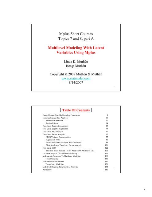
Mplus Short CoursesTopics 7 and 8, part AMultilevel Modeling With LatentVariables Using MplusLinda K. MuthénBengt MuthénCopyright © 2008 Muthén & Muthénwww.statmodel.com8/14/20071Table Of ContentsGeneral Latent Variable Modeling FrameworkComplex Survey Data AnalysisIntraclass CorrelationDesign EffectsTwo-Level Regression AnalysisTwo-Level Logistic RegressionTwo-Level Path AnalysisTwo-Level Factor AnalysisSIMS Variance DecompositionAggression ItemsTwo-Level Factor Analysis With CovariatesMultiple Group, Two-Level Factor AnalysisTwo-Level SEMPractical Issues Related To The Analysis Of Multilevel DataTechnical Aspects Of Multilevel ModelingMultivariate Approach To Multilevel ModelingTwin ModelingMultilevel Growth ModelsThree-Level ModelingMultilevel Discrete-Time Survival AnalysisReferences41112142344506577828610612213313614515015215617518021

Several programs in one• Structural equation modeling• Item response theory analysis• Latent class analysis• Latent transition analysis• Survival analysis• Multilevel analysis• Complex survey data analysis• Monte Carlo simulationMplusFully integrated in the general latent variable framework5Continuous ObservedAnd Latent VariablesAdding CategoricalObserved And LatentVariablesOverviewSingle-Level AnalysisCross-SectionalDay 1Regression AnalysisPath AnalysisExploratory Factor AnalysisConfirmatory Factor AnalysisStructural Equation ModelingDay 3Regression AnalysisPath AnalysisExploratory Factor AnalysisConfirmatory Factor AnalysisStructural Equation ModelingLatent Class AnalysisFactor Mixture AnalysisStructural Equation MixtureModelingLongitudinalDay 2Growth AnalysisDay 4Latent Transition AnalysisLatent Class Growth AnalysisGrowth AnalysisGrowth Mixture ModelingDiscrete-Time SurvivalMixture AnalysisMissing Data Analysis63

Overview (Continued)Multilevel AnalysisContinuous ObservedAnd Latent VariablesAdding CategoricalObserved And LatentVariablesCross-SectionalDay 5Regression AnalysisPath AnalysisExploratory Factor AnalysisConfirmatory Factor AnalysisStructural Equation ModelingDay 5Latent Class AnalysisFactor Mixture AnalysisLongitudinalDay 5Growth AnalysisDay 5Growth Mixture Modeling7Analysis With Multilevel DataUsed when data have been obtained by cluster samplingand/or unequal probability sampling to avoid biases inparameter estimates, standard errors, and tests of model fitand to learn about both within- and between-clusterrelationships.Analysis Considerations• Sampling perspective• Aggregated modeling – SUDAAN• TYPE = COMPLEX– Clustering, sampling weights, stratification(Asparouhov, 2005)84

Analysis With Multilevel Data (Continued)• Multilevel perspective• Disaggregated modeling – multilevel modeling• TYPE = TWOLEVEL– Clustering, sampling weights, stratification• Multivariate modeling• TYPE = GENERAL– Clustering, sampling weights, stratification• Combined sampling and multilevel perspective• TYPE = COMPLEX TWOLEVEL• Clustering, sampling weights, stratification9Analysis With Multilevel Data (Continued)Analysis Areas• Multilevel regression analysis• Multilevel path analysis• Multilevel factor analysis• Multilevel SEM• Multilevel growth modeling• Multilevel latent class analysis• Multilevel latent transition analysis• Multilevel growth mixture modeling105

Complex Survey Data Analysis11Intraclass CorrelationConsider nested, random-effects ANOVA for unit i in cluster j,y ij = v + η j + ε ij ; i = 1, 2,…, n j ; j = 1,2,…, J. (44)Random sample of J clusters (e.g. schools).With timepoint as i and individual as j, this is a repeatedmeasures model with random intercepts.Consider the covariance and variances for cluster members i = kand i = l,Coυ(y kj , y lj ) = V(η), (45)V(y kj ) = V(y lj ) = V(η) + V(ε), (46)resulting in the intraclass correlationρ(y kj , y lj ) = V(η)/[V(η) + V(ε)]. (47)Interpretation: Between-cluster variability relative to totalvariation, intra-cluster homogeneity.126

NLSY Household ClustersHousehold # of Households* Intraclass Correlations for SiblingsType(# of respondents) Year Heavy DrinkingSingleTwoThreeFourFiveSix5,9441,9856341703251982198319841985198819890.190.180.120.090.040.06Total number of households: 8,770Total number of respondents: 12,686Average number of respondents per household: 1.4*Source: NLS User’s Guide, 1994, p.24713Design EffectsConsider cluster sampling with equal cluster sizes and thesampling variance of the mean.V C : correct variance under cluster samplingV SRS : variance assuming simple random samplingV C ≥ V SRS but cluster sampling more convenient, lessexpensive.DEFF = V C / V SRS = 1 + (s –1) ρ, (47)where s is the common cluster size and ρ is the intraclasscorrelation (common range: 0.00 – 0.50).147

Random Effects ANOVA Example200 clusters of size 10 with intraclass correlation 0.2 analyzedas:• TYPE = TWOLEVEL• TYPE = COMPLEX• Regular analysis, ignoring clusteringDEFF = 1 + 9 * 0.2 = 2.815Input For Two-LevelRandom Effects ANOVA AnalysisTITLE:DATA:VARIABLE:ANALYSIS:MODEL:Random effects ANOVA dataTwo-level analysis with balanced dataFILE = anova.dat;NAMES = y cluster;USEV = y;CLUSTER = cluster;TYPE = TWOLEVEL;%WITHIN%y;%BETWEEN%y;168

Output Excerpts Two-LevelRandom Effects ANOVA AnalysisModel ResultsWithin LevelEstimatesS.E.Est./S.E.VariancesYBetween Level0.7790.02531.293MeansY0.0030.0380.076VariancesY0.2120.0287.49617Input For ComplexRandom Effects ANOVA AnalysisTITLE:DATA:VARIABLE:ANALYSIS:Random effects ANOVA dataComplex analysis with balanced dataFILE = anova.dat;NAMES = y cluster;USEV = y;CLUSTER = cluster;TYPE = COMPLEX;189

Output Excerpts ComplexRandom Effects ANOVA AnalysisModel ResultsMeansYEstimates0.003S.E.0.038Est./S.E.0.076VariancesY0.9900.03627.53819Input For Random Effects ANOVA AnalysisIgnoring ClusteringTITLE:DATA:VARIABLE:!ANALYSIS:Random effects ANOVA dataIgnoring clusteringFILE = anova.dat;NAMES = y cluster;USEV = y;CLUSTER = cluster;TYPE = MEANSTRUCTURE;2010

Output Excerpts Random EffectsANOVA Analysis Ignoring ClusteringModel ResultsMeansYEstimates0.003S.E.0.022Est./S.E.0.131VariancesY0.9900.03131.623Note: The estimated mean has SE = 0.022 instead of the correct 0.03821Further Readings On Complex Survey DataAsparouhov, T. (2005). Sampling weights in latent variable modeling.Structural Equation Modeling, 12, 411-434.Chambers, R.L. & Skinner, C.J. (2003). Analysis of survey data.Chichester: John Wiley & Sons.Kaplan, D. & Ferguson, A.J (1999). On the utilization of sampleweights in latent variable models. Structural Equation Modeling, 6,305-321.Korn, E.L. & Graubard, B.I (1999). Analysis of health surveys. NewYork: John Wiley & Sons.Patterson, B.H., Dayton, C.M. & Graubard, B.I. (2002). Latent classanalysis of complex sample survey data: application to dietary data.Journal of the American Statistical Association, 97, 721-741.Skinner, C.J., Holt, D. & Smith, T.M.F. (1989). Analysis of complexsurveys. West Sussex, England: Wiley.Stapleton, L. (2002). The incorporation of sample weights intomultilevel structural equation models. Structural EquationModeling, 9, 475-502.2211

Two-Level Regression Analysis23Cluster-Specific RegressionsIndividual i in cluster j(1) y ij = ß 0j + ß 1j x ij + r ij (2a) ß 0j = γ 00 + γ 01 w j + u 0j(2b) ß 1j = γ 10 + γ 11 w j + u 1jβ 0yj = 1j = 2j = 3β 1wxw2412

Two-Level Regression Analysis With RandomIntercepts And Random Slopes In Multilevel TermsTwo-level analysis (individual i in cluster j):y ijx ijw j: individual-level outcome variable: individual-level covariate: cluster-level covariateRandom intercepts, random slopes:Level 1 (Within) : y ij = ß 0j + ß 1j x ij + r ij , (1)Level 2 (Between) : ß 0j = γ 00 + γ 01 w j + u 0j , (2a)Level 2 (Between) : ß 1j = γ 10 + γ 11 w j + u 1j . (2b)• Mplus gives the same estimates as HLM/MLwiN ML (not REML):• V (r) (residual variance for level 1)• γ 00 , γ 01 , γ 10 , γ 11 , V(u 0 ), V(u 1 ), Cov(u 0 , u 1 )• Centering of x: subtracting grand mean or group (cluster) mean25NELS Data• The data—National Education Longitudinal Study(NELS:88)• Base year Grade 8—followed up in Grades 10 and 12• Students sampled within 1,035 schools—approximately26 students per school, n = 14,217• Variables—reading, math, science, history-citizenshipgeography,and background variables2613

NELS Math Achievement RegressionWithinBetweenfemalestud_sess1s2m92per_advaprivatecatholicm92s1s2mean_ses27Input For NELS Math Achievement RegressionTITLE:DATA:NELS math achievement regressionFILE IS completev2.dat;! National Education Longitudinal Study (NELS)FORMAT IS f8.0 12f5.2 f6.3 f11.4 23f8.2f18.2 f8.0 4f8.2;VARIABLE: NAMES ARE school r88 m88 s88 h88 r90 m90 s90 h90 r92m92 s92 h92 stud_ses f2pnlwt transfer minor coll_aspalgebra retain aca_back female per_mino hw_timesalary dis_fair clas_dis mean_col per_high unsafenum_frie teaqual par_invo ac_track urban size ruralprivate mean_ses catholic stu_teac per_adva tea_excetea_res;USEV = m92 female stud_ses per_adva private catholicmean_ses;!per_adva = percent teachers with an MA or higherWITHIN = female stud_ses;BETWEEN = per_adva private catholic mean_ses;MISSING = blank;CLUSTER = school;CENTERING = GRANDMEAN (stud_ses per_adva mean_ses);2814

Input For NELS Math Achievement Regression(Continued)ANALYSIS: TYPE = TWOLEVEL RANDOM MISSING;MODEL:OUTPUT:%WITHIN%s1 | m92 ON female;s2 | m92 ON stud_ses;%BETWEEN%m92 s1 s2 ON per_adva private catholic mean_ses;m92 WITH s1 s2;TECH8 SAMPSTAT;29Summary of DataOutput Excerpts NELS MathAchievement RegressionNumber of clusters 902N = 10,933Size (s)Cluster ID with Size s12345898634174345706540740402665123164650959846192081446494717586281263271596140793469681531090444395938597479183234526544502511662830489858285508935699531735719182196825419952679087842426406859526234380636411267574104686802832661602813845441412115178339086733508802004872193707188923982860677081754360835661257738134139976163496562145624183085754987440051670128352578415773684221474396858106920770109104755580675877458543015

Output Excerpts NELS MathAchievement Regression (Continued)222324252627283031323436424379570 15426 97947 93599 85125 10926 46036411 60328 70024 6783536988 22874 50626 1909156619 59710 34292 18826 6220944586 67832 1651582887847 769093617712786 53660 47120 94802805535327289842 315729951675115Average cluster size 12.187Estimated Intraclass Correlations for the Y VariablesIntraclassVariable CorrelationM92 0.10731Output Excerpts NELS MathAchievement Regression (Continued)Tests of Model FitLoglikelihoodH0 Value -39390.404Information CriteriaNumber of Free parameters 21Akaike (AIC) 78822.808Bayesian (BIC) 78976.213Sample-Size Adjusted BIC 78909.478(n* = (n + 2) / 24)Model ResultsWithin LevelResidualVariancesM92Between LevelS1ONPER_ADVAPRIVATECATHOLICMEAN_SESEstimates S.E. Est./S.E.70.5770.084-0.134-0.736-0.2321.1490.8410.8440.7800.42861.4420.100-0.159-0.944-0.5423216

Cross-Level Influence (Continued)Cross-level interaction, or between-level (level 2) variablemoderating a within level (level 1) relationship:Random slopey ij = β 0 + β 1j x ij + r ijMplus:MODEL:β 1j = γ 10 + γ 11 w j + u 1j%WITHIN%;beta1 | y ON x;%BETWEEN%;beta1 ON w;! estimates gamma1135Random Slopes• In single-level modeling random slopes ß i describe variation acrossindividuals i,y i = α i + ß i x i + ε i , (100)α i = α + ζ 0i , (101)ß i = ß + ζ 1i , (102)resulting in heteroscedastic residual variances2V ( y i | x i )= V ( ß i ) xi+ θ . (103)• In two-level modeling random slopes ß j describe variation acrossclusters jy ij = a j + ß j x ij + ε ij , (104)a j = a + ζ 0j , (105)ß j = ß+ ζ 1j , (106)A small variance for a random slope typically leads to slow convergence of theML-EM iterations. This suggests respecifying the slope as fixed.Mplus allows random slopes for predictors that are• Observed covariates• Observed dependent variables36• Continuous latent variables18

Further Readings OnMultilevel Regression AnalysisLudtke Marsh, Robitzsch, Trautwein, Asparouhov, Muthen(2007). Analysis of group level effects using multilevel modeling:Probing a latent covariate approach. Submitted for publication.Raudenbush, S.W. & Bryk, A.S. (2002). Hierarchical linear models:Applications and data analysis methods. Second edition. NewburyPark, CA: Sage Publications.Snijders, T. & Bosker, R. (1999). Multilevel analysis. An introductionto basic and advanced multilevel modeling. Thousand Oakes, CA:Sage Publications.37Logistic And Probit Regression3819

Categorical Outcomes: Logit And Probit RegressionProbability varies as a function of x variables (here x 1 , x 2 )P(u = 1 | x 1 , x 2 ) = F[β 0 + β 1 x 1 + β 2 x 2 ], (22)P(u = 0 | x 1 , x 2 ) = 1 - P[u = 1 | x 1 , x 2 ], where F[z] is either thestandard normal (Φ[z]) or logistic (1/[1 + e -z ]) distributionfunction.Example: Lung cancer and smoking among coal minersu lung cancer (u = 1) or not (u = 0)x 1 smoker (x 1 = 1), non-smoker (x 1 = 0)x 2 years spent in coal mine39Categorical Outcomes: Logit And Probit RegressionP(u = 1 | x 1 , x 2 ) = F [β 0 + β 1 x 1 + β 2 x 2 ], (22)1P( u = 1 x 1 , x 2 )x 1 = 1Probit / Logitx 1 = 1x 1 = 0x 1 = 00.50x 2x 24020

Interpreting Logit And Probit Coefficients• Sign and significance• Odds and odds ratios• Probabilities41Logistic Regression And Log OddsOdds (u = 1 | x) = P(u = 1 | x)/ P(u = 0 | x)= P(u = 1 | x) / (1 – P(u = 1 | x)).The logistic functionP ( u = 1 | x)=1+egives a log odds linear in x,logit = log [odds (u = 1 | x)] = log [P(u = 1 | x) / (1 – P(u = 1 | x))]= log= log= log1- ( β 0 + β1x)⎡ 11⎢/ (1 −− β +− +⎣1+0 β1x)( βe1+e 0 β1⎡ − ( β+ 0 + β1x)1 1 e ⎤⎢*− ( β + ) − ( + ) ⎥⎢⎣1+0 β1x β0β1xee⎥⎦( x )( β x)[ e 0 + β1] = β + β x01⎤) ⎥⎦4221

Logistic Regression And Log Odds (Continued)• logit = log odds = β 0 + β 1 x• When x changes one unit, the logit (log odds) changes β 1 units• When x changes one unit, the odds changese β 1 units43Two-Level Logistic RegressionWith j denoting cluster,logit ij = log (P(u ij = 1)/P(u ij = 0)) = α j + β j * x ijwhereα j = α + u 0jβ j = β + u 1jHigh/low α j value means high/low logit (high log odds)4422

Predicting Juvenile DelinquencyFrom First Grade Aggressive Behavior• Cohort 1 data from the Johns Hopkins University PreventiveIntervention Research Center• n= 1,084 students in 40 classrooms, Fall first grade• Covariates: gender and teacher-rated aggressive behavior45Input For Two-Level Logistic RegressionTITLE:Hopkins Cohort 1 2-level logistic regressionDATA:FILE = Cohort1_classroom_ALL.DAT;VARIABLE:NAMES = prcid juv99 gender stub1F bkRule1F harmO1FbkThin1F yell1F takeP1F fight1F lies1Ftease1F;CLUSTER = classrm;USEVAR = juv99 male aggress;CATEGORICAL = juv99;MISSING = ALL (999);WITHIN = male aggress;DEFINE:male = 2 - gender;aggress = stub1F + bkRule1F + harmO1F + bkThin1F +yell1F + takeP1F + fight1F + lies1F + tease1F;4623

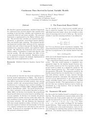
Input For Two-Level Logistic Regression(Continued)ANALYSIS:TYPE = TWOLEVEL MISSING;PROCESS = 2;MODEL:%WITHIN%juv99 ON male aggress;%BETWEEN%OUTPUT:TECH1 TECH8;47Output Excerpts Two-Level Logistic RegressionMODEL RESULTSEstimatesS.EEst./S.E.Within LevelJUV99MALEON1.0710.1497.193AGGRESS0.0600.0106.191Between LevelThresholdsJUV99$12.9810.20514.562VariancesJUV990.8070.2503.2284824

Understanding The Between-LevelIntercept Variance• Intra-class correlation– ICC = 0.807/(π 2 /3 + 0.807)• Odds ratios– Larsen & Merlo (2005). Appropriate assessment of neighborhoodeffects on individual health: Integrating random and fixed effects inmultilevel logistic regression. American Journal ofEpidemiology, 161, 81-88.– Larsen proposes MOR:"Consider two persons with the same covariates, chosen randomly fromtwo different clusters. The MOR is the median odds ratio between theperson of higher propensity and the person of lower propensity."MOR = exp( √(2* σ 2 ) * Φ -1 (0.75) )In the current example, ICC = 0.20, MOR = 2.36• Probabilities– Compare α j =1 SD and α k =-1 SD from the mean49Two-Level Path Analysis5025

A Path Model With A Binary OutcomeAnd A Mediator With Missing DataLogistic RegressionPath Modelfemalemothedhomeresexpectlunchexpelarrestdroptht7hispblackmath7math10hsdropfemalemothedhomeresexpectlunchexpelarrestdroptht7hispblackmath7math10hsdrop51Two-Level Path AnalysisWithinBetweenfemalemothedhomeresexpectlunchexpelarrestdroptht7hispblackmath7math10hsdropmath10hsdrop5226

Input For A Two-Level Path Analysis Model WithA Categorical Outcome And Missing Data OnThe Mediating VariableTITLE:DATA:VARIABLE:ANALYSIS:a twolevel path analysis with a categorical outcomeand missing data on the mediating variableFILE = lsayfull_dropout.dat;NAMES = female mothed homeres math7 math10 expelarrest hisp black hsdrop expect lunch droptht7schcode;MISSING = ALL (9999);CATEGORICAL = hsdrop;CLUSTER = schcode;WITHIN = female mothed homeres expect math7 lunchexpel arrest droptht7 hisp black;TYPE = TWOLEVEL MISSING;ESTIMATOR = ML;ALGORITHM = INTEGRATION;INTEGRATION = MONTECARLO (500);53Input For A Two-Level Path Analysis Model WithA Categorical Outcome And Missing Data OnThe Mediating Variable (Continued)MODEL:%WITHIN%hsdrop ON female mothed homeres expect math7 math10lunch expel arrest droptht7 hisp black;math10 ON female mothed homeres expect math7 lunchexpel arrest droptht7 hisp black;%BETWEEN%hsdrop*1; math10*1;OUTPUT:PATTERNS SAMPSTAT STANDARDIZED TECH1 TECH8;5427

Output Excerpts A Two-Level Path Analysis ModelWith A Categorical Outcome And Missing DataOn The Mediating VariableSummary Of DataNumber of patterns 2Number of clusters 44Size (s)1213363839404142434445Cluster ID with Size s30430530710613810330814610230314112211210912010114355Output Excerpts A Two-Level Path Analysis ModelWith A Categorical Outcome And Missing DataOn The Mediating Variable (Continued)Size (s)Cluster ID with Size s46474950515253555714414010812612713714214513511112411713112310511014711830113658121591197310489302931183091155628

Output Excerpts A Two-Level Path Analysis ModelWith A Categorical Outcome And Missing DataOn The Mediating Variable (Continued)Model ResultsWithin LevelHSDROP ONFEMALEMOTHEDHOMERESEXPECTMATH7MATH10LUNCHEXPELARRESTDROPTHT7HISPBLACKEstimates0.323-0.253-0.077-0.244-0.011-0.0310.0080.9470.0680.757-0.118-0.086S.E.0.1710.1030.0550.0650.0150.0110.0060.2250.3210.2840.2740.253Est./S.E.1.887-2.457-1.401-3.756-0.754-2.7061.3244.2010.2122.665-0.431-0.340Std0.323-0.253-0.077-0.244-0.011-0.0310.0080.9470.0680.757-0.118-0.086StdYX0.077-0.121-0.061-0.159-0.055-0.1970.0740.1210.0070.074-0.016-0.01357Output Excerpts A Two-Level Path Analysis ModelWith A Categorical Outcome And Missing DataOn The Mediating Variable (Continued)EstimatesS.E.Est./S.E.StdStdYXMATH10 ONFEMALEMOTHEDHOMERESEXPECTMATH7LUNCHEXPELARRESTDROPTHT7HISPBLACK-0.8410.2630.5680.9850.940-0.039-1.293-3.426-1.424-0.501-0.3690.3980.2150.1360.1620.0230.0170.8251.0221.0490.7280.733-2.1101.2224.1696.09140.123-2.308-1.567-3.353-1.358-0.689-0.503-0.8410.2630.5680.9850.940-0.039-1.293-3.426-1.424-0.501-0.369-0.0310.0200.0700.1000.697-0.059-0.026-0.054-0.022-0.010-0.0095829

Output Excerpts A Two-Level Path Analysis ModelWith A Categorical Outcome And Missing DataOn The Mediating Variable (Continued)EstimatesS.E.Est./S.E.StdStdYXResidual VariancesMATH1062.0102.16228.68362.0100.341Between LevelMeansMATH10ThresholdsHSDROP$1VariancesHSDROPMATH1010.226-1.0760.2863.7571.3400.5600.1331.2487.632-1.9202.1503.01110.2260.2863.7575.2761.0001.00059Two-Level Mediationa jmb jxc’ jyIndirect effect:α + β + Cov (a j , b j )Bauer, Preacher & Gil (2006). Conceptualizing and testing randomindirect effects and moderated mediation in multilevel models: Newprocedures and recommendations. Psychological Methods, 11, 142-163.6030

Input For Two-Level MediationMONTECARLO:NAMES ARE y m x;WITHIN = x;NOBSERVATIONS = 1000;NCSIZES = 1;CSIZES = 100 (10);NREP = 100;MODEL POPULATION:%WITHIN%c | y ON x;b | y ON m;a | m ON x;x*1; m*1; y*1;%BETWEEN%y WITH m*0.1 b*0.1 a*0.1 c*0.1;m WITH b*0.1 a*0.1 c*0.1;a WITH b*0.1 c*0.1;b WITH c*0.1;y*1 m*1 a*1 b*1 c*1;[a*0.4 b*0.5 c*0.6];61Input For Two-Level Mediation (Continued)ANALYSIS:TYPE = TWOLEVEL RANDOM;MODEL:%WITHIN%c | y ON x;b | y ON m;a | m ON x;m*1; y*1;%BETWEEN%y WITH M*0.1 b*0.1 a*0.1 c*0.1;m WITH b*0.1 a*0.1 c*0.1;a WITH b*0.1 (cab);a WITH c*0.1;b WITH c*0.1;y*1 m*1 a*1 b*1 c*1;[a*0.4] (ma);[b*0.5] (mb);[c*0.6];MODEL CONSTRAINT:NEW(m*0.3);m=ma*mb+cab;6231

32630.1100.9100.01930.13120.13760.07560.100C0.1500.9200.01370.11010.11740.09640.100BWITHA0.1600.9700.01320.11650.11470.11380.100C0.0700.9500.01190.11160.10810.08150.100A0.1200.9400.01050.10850.10290.10330.100BWITHM0.0900.9400.01260.12370.11210.08680.100C0.1900.9100.01730.11620.13180.10860.100A0.2100.9100.01580.1140.12460.12120.100BWITHYBetween Level1.0000.9100.00290.04960.05381.00111.000M1.0000.9600.00280.05300.05301.00201.000YResidualvariancesWithin LevelCoeffCoverAverageStd.Dev.AveragePopulation% Sig95%M. S. E.S.E.EstimatesOutput Excerpts Two Level Mediation640.5500.9500.02010.13160.14220.29040.300MNew/Additional Parameters1.0000.9500.02390.15870.15411.01881.000A1.0000.9500.02120.15450.14430.97681.000B1.0000.9800.02010.17180.14130.98021.000C1.0000.9300.03160.15710.17821.01131.000M1.0000.9100.02800.16890.16811.00711.000YVariances0.9700.9700.00960.10720.09720.38540.400A1.0000.8900.01620.10610.12790.50220.500B1.0000.9300.01500.11250.12290.59790.600C0.0500.9500.01200.10560.1102-0.00310.000M0.0500.9500.01320.11130.11510.00700.000YMeans0.1400.9400.01780.12850.13420.10340.100MWITHY0.0700.9600.01120.11560.10560.08920.100CWITHBOutput Excerpts Two-Level Mediation (Continued)

Two-Level Factor Analysis65Two-Level Factor Analysis• Recall random effects ANOVA (individual i in cluster j ):y ij = ν + η j + ε ij = y B + y W• Two-level factor analysis (r = 1, 2, …, p items):jijy rij = ν r + λ B η B + ε Br j rj r(between-clustervariation)+ λ W η Wij + ε Wrij(within-clustervariation)6633

Two-Level Factor Analysis (Continued)• Covariance structure:V(y) = V(y B )+ V(y w ) = Σ B + Σ w ,Σ B = Λ B Ψ B Λ B + Θ B ,Σ W = Λ W Ψ W Λ W + Θ W .• Two interpretations:– variance decomposition, including decomposing theresidual– random intercept model67Two-Level Factor Analysis And Design EffectsMuthén & Satorra (1995; Sociological Methodology): MonteCarlo study using two-level data (200 clusters of varying sizeand varying intraclass correlations), a latent variable modelwith 10 variables, 2 factors, conventional ML using theregular sample covariance matrix S T , and 1,000 replications (d.f. = 34).Λ B = Λ W =11111000000000011111Ψ B , Θ B reflecting different icc’sy ij= ν + Λ(η B+ η W) + ε B+ εj ij j W ijV(y) = Σ B + Σ W = Λ(Ψ B + Ψ W ) Λ + Θ B + Θ W6834

Two-Level Factor Analysis And Design Effects (Continued)Inflation of χ 2 due to clusteringIntraclassCorrelation0.050.100.20Chi-square meanChi-square var5%1%Chi-square meanChi-square var5%1%Chi-square meanChi-square var5%1%Cluster Size7 15 30 6035685.61.436758.51.04210023.58.636727.61.6408916.05.25215257.735.0388010.62.84611737.617.67330293.183.1419620.47.75818973.652.111473499.999.469Two-Level Factor Analysis And Design Effects (Continued)• Regular analysis, ignoring clustering• Inflated chi-square, underestimated SE’s• TYPE = COMPLEX• Correct chi-square and SE’s but only if model aggregates,e.g. Λ B = Λ W• TYPE = TWOLEVEL• Correct chi-square and SE’s7035

Two-Level Factor Analysis (IRT)WithinBetweenu1 u2 u3 u4u1 u2 u3 u4fwfbu* ij= λ ( f B+ f w) + εj ij ij71Input For A Two-Level Factor Analysis (IRT)Model With Categorical OutcomesTITLE:DATA:VARIABLE:ANALYSIS:MODEL:this is an example of a two-level factor analysismodel with categorical outcomesFILE = catrep1.dat;NAMES ARE u1-u6 clus;CATEGORICAL = u1-u6;CLUSTER = clus;TYPE = TWOLEVEL;ESTIMATION = ML;ALGORITHM = INTEGRATION;%WITHIN%fw BY u1@1u2 (1)u3 (2)u4 (3)u5 (4)u6 (5);7236

Input For A Two-Level Factor Analysis (IRT)Model With Categorical Outcomes (Continued)OUTPUT:%BETWEEN%fb BY u1@1u2 (1)u3 (2)u4 (3)u5 (4)u6 (5);TECH1 TECH8;73Output Excerpts A Two-Level Factor Analysis(IRT) Model With Categorical OutcomesTests Of Model FitLoglikelihoodH0 ValueInformation CriteriaNumber of Free ParametersAkaike (AIC)Bayesian (BIC)Sample-Size Adjusted BIC(n* = (n + 2) / 24)-3696.117137418.2357481.5057440.2177437

Output Excerpts A Two-Level Factor Analysis(IRT) Model With Categorical Outcomes(Continued)Model ResultsWithin LevelFW BYU1U2U3U4U5U6Estimates1.0000.9151.0871.0581.1911.143S.E.0.0000.1460.1690.1640.1850.178Est./S.E.0.0006.2646.4376.4416.4496.439VariancesFW0.8340.1914.36075Output Excerpts Two-Level Factor Analysis(IRT) Model With Categorical Outcomes (Continued)Between LevelFB BYU1U2U3U4U5U6Estimates1.0000.9151.0871.0581.1911.143S.E.0.0000.1460.1690.1640.1850.178Est./S.E.0.0006.2646.4376.4416.4496.439ThresholdsU1$1U2$1U3$1U4$1U5$1U6$1-0.2060.001-0.016-0.064-0.033-0.0210.0960.0910.1000.0980.1050.102-2.1500.007-0.156-0.652-0.315-0.209VariancesFB0.4960.1393.5627638

SIMS Variance DecompositionThe Second International Mathematics Study (SIMS; Muthén,1991, JEM).• National probability sample of school districts selectedproportional to size; a probability sample of schoolsselected proportional to size within school district, and twoclasses randomly drawn within each school• 3,724 students observed in 197 classes from 113 schoolswith class sizes varying from 2 to 38; typical class size ofaround 20• Eight variables corresponding to various areas of eighthgrademathematics• Same set of items administered as a pretest in the Fall ofeighth grade and as a posttest in the Spring.77SIMS Variance Decomposition (Continued)Muthén (1991). Multilevel factor analysis of class and studentachievement components. Journal of Educational Measurement, 28,338-354.• Research questions: “The substantive questions of interest inthis article are the variance decomposition of the subscores withrespect to within-class student variation and between-classvariation and the change of this decomposition from pretest toposttest. In the SIMS … such variance decomposition relates tothe effects of tracking and differential curricula in eighth-grademath. On the one hand, one may hypothesize that effects ofselection and instruction tend to increase between-classvariation relative to within-class variation, assuming that theclasses are homogeneous, have different performance levels tobegin with, and show faster growth for higher initialperformance level. On the other hand, one may hypothesize thateighth-grade exposure to new topics will increase individualdifferences among students within each class so that posttestwithin-class variation will be sizable relative to posttestbetween-class variation.”7839

SIMS Variance Decomposition (Continued)y rij = ν r + λ Br η Bj + ε Brj + λ wr η wij + ε wrijV(y rij ) =BF + BE + WF + WEBetween reliability: BF / (BF + BE)– BE often small (can be fixed at 0)Within reliability: WF / (WF + WE)– sum of a small number of items gives a large WEIntraclass correlation:ICC = (BF + BE) / (BF + BE + WF+ WE)Large measurement error large WE small ICCTrue ICC = BF / (BF + WF)79Betweenfb_prerpp_prefract_preeqexp_preintnum_pretesti_preaeravol_precoorvis_prepfigure_preWithinfw_prefb_postrpp_postfract_posteqexp_postintnum_posttesti_postaeravol_postcoorvis_postfw_postpfigure_post8040

Table 4: Variance Decomposition of SIMS Achievement Scores(percentages of total variance in parenthesis)RPPFRACTNumberof Items Between Within881.542(34.0)1.460(38.2)Pretest2.990(66.0) .342.366(61.8)ANOVAProp-Between Between Within.382.084(38.5)1.906(40.8)PosttestProp-Between3.326(61.5) .382.767(59.2).41% IncreaseIn VarianceFACTOR ANALYSISError-freeProp. BetweenError-free% IncreaseIn VarianceBetween Within Pre Post Between Within35 11 .54 .52 29 4131 17 .60 .58 29 41EQEXP6.543(26.9)1.473(73.1).271.041(38.7)1.646(61.3).3992 18 .65 .64 113 117INTNUM2.127(25.2).358(70.9).29.195(30.6).442(69.4).3154 24 .63 .61 29 41TESTI5.580(33.3)1.163(66.7).33.664(34.5)1.258(65.5).3415 8.58 .5629 41AREAVOL2.094(17.2).451(82.8).17.156(24.1).490(75.9).2466 9.54 .5229 41COORVIS3.173(20.9).656(79.1).21.275(28.7).680(68.3).3259 4.57 .5529 41PFIGURE5.363(22.9)1.224(77.1).23.711(42.9)1.451(67.1).3396 19.60 .5487 13681Second-Generation JHU PIRC Trial Aggression ItemsItem Distributions for Cohort 3: Fall 1st Grade (n=362 males in 27 classrooms)AlmostNeverRarelySometimesOftenVery OftenAlmostAlwaysStubborn(scored as 1)42.5(scored as 2)21.3(scored as 3)18.5(scored as 4)7.2(scored as 5)6.4(scored as 6)4.1Breaks Rules37.616.022.77.58.38.0Harms Others69.312.49.403.92.52.5Breaks Things79.86.605.203.93.60.8Yells at Others61.914.111.95.84.12.2Takes Others’PropertyFights72.960.59.7013.810.813.52.55.52.23.01.93.6Harms Property74.99.909.102.82.80.6Lies72.412.48.002.83.31.1Talks Back toAdultsTeases Classmates79.655.09.7014.47.8017.71.47.20.84.41.41.4Fights WithClassmatesLoses Temper67.461.612.415.510.213.85.04.73.33.01.71.48241

Hypothesized Aggressiveness Factors• Verbal aggression– Yells at others– Talks back to adults– Loses temper– Stubborn• Property aggression– Breaks things– Harms property– Takes others’ property– Harms others• Person aggression– Fights– Fights with classmates– Teases classmates83Two-Level Factor AnalysisWithiny1 y2 y3 y4 y5 y6y7 y8 y9 y10 y11 y12 y13fw1fw2fw3Betweeny1 y2 y3 y4 y5 y6y7 y8 y9 y10 y11 y12y13fb1fb2fb38442

Promax Rotated LoadingsStubbornBreaks RulesHarms OthersBreaks ThingsYells at OthersTakes Others' PropertyFightsHarms PropertyLiesTalks Back to AdultsTeases ClassmatesFights With ClassmatesLoses TemperWithin-Level Loadings1 2 30.07 0.70 0.050.25 0.31 0.370.52 0.16 0.270.84 0.16 -0.010.15 0.64 0.130.57 0.00 0.370.20 0.21 0.630.73 0.21 0.100.48 0.28 0.240.29 0.71 0.230.11 0.19 0.620.10 0.31 0.630.12 0.75 0.04Between-Level Loadings1 2 3-0.19 1.03 0.070.15 0.28 0.310.35 -0.20 0.720.71 0.01 0.410.38 0.74 -0.010.86 -0.04 0.120.09 0.03 0.890.90 -0.05 0.160.86 0.33 -0.210.41 0.58 -0.040.37 0.31 0.30-0.19 0.38 0.880.17 0.78 0.1285Two-Level Factor Analysis With Covariates8643

Two-Level Factor Analysis With CovariatesWithinBetweeny1y1x1fw1y2y2y3y4wfby3y4x2fw2y5y5y6y687Input For Two-Level Factor AnalysisWith CovariatesTITLE:DATA:VARIABLE:ANALYSIS:MODEL:this is an example of a two-level CFA withcontinuous factor indicators with two factors on thewithin level and one factor on the between levelFILE IS ex9.8.dat;NAMES ARE y1-y6 x1 x2 w clus;WITHIN = x1 x2;BETWEEN = w;CLUSTER IS clus;TYPE IS TWOLEVEL;%WITHIN%fw1 BY y1-y3;fw2 BY y4-y6;fw1 ON x1 x2;fw2 ON x1 x2;%BETWEEN%fb BY y1-y6;fb ON w;8844

Input For Monte Carlo Simulations ForTwo-Level Factor Analysis With CovariatesTITLE:MONTECARLO:ANALYSIS:This is an example of a two-level CFA withcontinuous factor indicators with twofactors on the within level and one factoron the between levelNAMES ARE y1-y6 x1 x2 w;NOBSERVATIONS = 1000;NCSIZES = 3;CSIZES = 40 (5) 50 (10) 20 (15);SEED = 58459;NREPS = 1;SAVE = ex9.8.dat;WITHIN = x1 x2;BETWEEN = w;TYPE = TWOLEVEL;89Input For Monte Carlo Simulations ForTwo-Level Factor Analysis With Covariates(Continued)MODEL POPULATION:%WITHIN%x1-x2@1;fw1 BY y1@1 y2-y3*1;fw2 BY y4@1 y5-y6*1;fw1-fw2*1;y1-y6*1;fw1 ON x1*.5 x2*.7;fw2 ON x1*.7 x2*.5;%BETWEEN%[w@0]; w*1;fb BY y1@1 y2-y6*1;y1-y6*.3;fb*.5;fb ON w*1;9045

Input For Monte Carlo Simulations ForTwo-Level Factor Analysis With Covariates(Continued)MODEL:%WITHIN%OUTPUT:fw1 BY y1@1 y2-y3*1;fw2 BY y4@1 y5-y6*1;fw1-fw2*1;y1-y6*1;fw1 ON x1*.5 x2*.7;fw2 ON x1*.7 x2*.5;%BETWEEN%fb BY y1@1 y2-y6*1;y1-y6*.3;fb*.5;fb ON w*1;TECH8 TECH9;91NELS Data• The data—National Education Longitudinal Study(NELS:88)• Base year Grade 8—followed up in Grades 10 and 12• Students sampled within 1,035 schools—approximately26 students per school, n = 14,217• Variables—reading, math, science, history-citizenshipgeography,and background variables• Data for the analysis—reading, math, science, historycitizenship-geography9246

NELS Two-Level Longitudinal Factor AnalysisWith CovariatesWithinBetweenr88 m88 s88 h88 r90 m90 s90 h90 r92 m92 s92 h92r88 m88 s88 h88 r90 m90 s90 h90 r92 m92 s92 h92fw1fw2fw3fb1fb2fb3femalestud_sesper_advaprivatecatholic mean_ses93Input For NELS Two-Level Longitudinal FactorAnalysis With CovariatesTITLE:DATA:VARIABLE:two-level factor analysis with covariates using the NELSdataFILE = NELS.dat;FORMAT = 2f7.0 f11.4 12f5.2 11f8.2;NAMES = id school f2pnlwt r88 m88 s88 h88 r90 m90 s90 h90r92 m92 s92 h92 stud_ses female per_mino urban size ruralprivate mean_ses catholic stu_teac per_adva;!Variable Description!m88 = math IRT score in 1988!m90 = math IRT score in 1990!m92 = math IRT score in 1992!r88 = reading IRT score in 1988!r90 = reading IRT score in 1990!r92 = reading IRT score in 19929447

Input For NELS Two-Level Longitudinal FactorAnalysis With Covariates (Continued)!s88 = science IRT score in 1988!s90 = science IRT score in 1990!s92 = science IRT score in 1992!h88 = history IRT score in 1988!h90 = history IRT score in 1990!h92 = history IRT score in 1992!female = scored 1 vs 0!stud_ses = student family ses in 1990 (f1ses)!per_adva = percent teachers with an MA or higher!private = private school (scored 1 vs 0)!catholic = catholic school (scored 1 vs 0)!private = 0, catholic = 0 implies public schoolMISSING = BLANK;CLUSTER = school;USEV = r88 m88 s88 h88 r90 m90 s90 h90 r92 m92 s92 h92female stud_ses per_adva private catholic mean_ses;WITHIN = female stud_ses;BETWEEN = per_adva private catholic mean_ses;95Input For NELS Two-Level Longitudinal FactorAnalysis With Covariates (Continued)ANALYSIS:MODEL:OUTPUT:TYPE = TWOLEVEL MISSING;%WITHIN%fw1 BY r88-h88;fw2 BY r90-h90;fw3 BY r92-h92;r88 WITH r90; r90 WITH r92; r88 WITH r92;m88 WITH m90; m90 WITH m92; m88 WITH m92;s88 WITH s90; s90 WITH s92;h88 WITH h90; h90 WITH h92;fw1-fw3 ON female stud_ses;%BETWEEN%fb1 BY r88-h88;fb2 BY r90-h90;fb3 BY r92-h92;fb1-fb3 ON per_adva private catholic mean_ses;SAMPSTAT STANDARDIZED TECH1 TECH8 MODINDICES;9648

Output Excerpts NELS Two-Level LongitudinalFactor Analysis With CovariatesSummary Of DataNumber of patterns 15Number of clusters 913Average cluster size 15.572Estimated Intraclass Correlations for the Y VariablesVariableIntraclassCorrelationVariableIntraclassCorrelationVariableIntraclassCorrelationR88H88S90M920.0670.1050.1100.111M88R90H90S920.1290.0760.1060.099S88M90R92H920.1000.1170.0730.09197Output Excerpts NELS Two-Level LongitudinalFactor Analysis With Covariates (Continued)Tests Of Model FitChi-Square Test of Model FitValueDegrees of FreedomP-ValueScaling Correction Factorfor MLR4883.539*1460.00001.046Chi-Square Test of Model Fit for the Baseline ModelValue150256.855Degrees of Freedom202P-Value0.0000CFI/TLICFITLI0.9680.956LoglikelihoodH0 ValueH1 Value-487323.777-484770.2579849

Output Excerpts NELS Two-Level LongitudinalFactor Analysis With Covariates (Continued)Information CriteriaNumber of Free ParametersAkaike (AIC)Bayesian (BIC)Sample-Size Adjusted BIC(n* = (n + 2) / 24)RMSEA (Root Mean Square Error Of Approximation)EstimateSRMR (Standardized Root Mean Square ResidualValue for BetweenValue for Within94974835.554975546.400975247.6760.0480.0410.02799Output Excerpts NELS Two-Level LongitudinalFactor Analysis With Covariates (Continued)Model ResultsEstimatesS.E.Est./S.E.StdStdYXWithin LevelFW1 BYR88M88S88H88FW2 BYR90M90S90H901.0000.9401.0051.0411.0000.9111.0030.9390.0000.0100.0100.0110.0000.0080.0100.0080.00094.85695.77897.8880.000109.67699.042113.6036.5286.1356.5596.7968.0387.3218.0657.5440.8120.8040.8370.8370.8420.8380.8590.85510050

Output Excerpts NELS Two-Level LongitudinalFactor Analysis With Covariates (Continued)FW3 BYR92M92S92H92FW1 ONFEMALESTUD_SESFW2 ONFEMALESTUD_SESFW3 ONFEMALESTUD_SES1.0000.9391.0030.934-0.4033.378-0.6214.169-1.0274.4180.0000.0090.0110.0090.1280.0960.1570.1100.1690.1220.000101.47390.276102.825-3.15035.264-3.94537.746-6.08736.1248.4607.9468.4827.905-0.0620.517-0.0770.519-0.1210.5220.8320.8450.8610.858-0.0310.418-0.0390.420-0.0640.422101Output Excerpts NELS Two-Level LongitudinalFactor Analysis With Covariates (Continued)Residual VariancesR88M88S88H88R90M90S90H90R92M92S92H92FW1FW2FW322.02120.61818.38319.80526.54622.75623.15021.00231.82125.21325.15522.47935.08153.07958.4380.3830.3380.3230.3700.4910.3750.3830.4030.6170.4850.5240.4890.6991.0051.24257.46461.00956.93953.58754.03360.74860.51652.12451.56252.01847.97446.01650.20152.80647.04122.02120.61818.38319.80526.54622.75623.15021.00231.82125.21325.15522.4790.8230.8220.8170.3410.3540.2990.3000.2910.2980.2620.2700.3080.2850.2590.2650.8230.8220.81710251

Output Excerpts NELS Two-Level LongitudinalFactor Analysis With Covariates (Continued)Between LevelFB1 BYR88M88S88H88FB2 BYR90M90S90H90FB3 BYR92M92S92H921.0001.5531.0611.0651.0001.4071.2200.9731.0001.4351.1600.9630.0000.0700.0580.0530.0000.0580.0620.0470.0000.0650.0650.0410.00022.13818.25519.9880.00024.40719.69720.4960.00022.09517.88923.2441.9523.0312.0712.0782.4133.3952.9432.3482.4723.5462.8682.3800.9330.9790.8870.8140.9231.0030.9460.8290.9470.9970.9380.871103Output Excerpts NELS Two-Level LongitudinalFactor Analysis With Covariates (Continued)Between LevelFB1 ONPER_ADVAPRIVATECATHOLICMEAN_SESFB2 ONPER_ADVAPRIVATECATHOLICMEAN_SESFB3 ONPER_ADVAPRIVATECATHOLICMEAN_SES0.2170.303-0.6962.5130.2800.453-0.5383.0540.4730.673-0.2063.1420.2920.3440.2770.2060.3380.3920.3340.2390.3750.4350.3720.2580.7420.883-2.51212.1850.8281.155-1.60912.8051.2611.547-0.55412.1690.1110.155-0.3571.2880.1160.188-0.2231.2660.1920.272-0.0841.2710.0240.042-0.0880.6720.0250.051-0.0550.6600.0410.074-0.0210.66310452

Output Excerpts NELS Two-Level LongitudinalFactor Analysis With Covariates (Continued)Residual VariancesR88M88S88H88R90M90S90H90R92M92S92H92FB1FB2FB30.5640.3991.1602.2031.017-0.0681.0252.5180.7060.0761.1201.8101.9793.0613.0100.1040.0930.1260.2030.1600.0550.1720.2160.1820.0760.1900.2110.2450.3450.4095.4374.2929.17010.8396.352-1.2255.94511.6363.8861.0005.9018.5998.0668.8757.3630.5640.3991.1602.2031.017-0.0681.0252.5180.7060.0761.1201.8100.5200.5260.4930.1290.0420.2130.3380.149-0.0060.1060.3130.1040.0060.1200.2420.5200.5260.493105Multiple-Group, Two-LevelFactor Analysis With Covariates10653

NELS Data• The data—National Education Longitudinal Study(NELS:88)• Base year Grade 8—followed up in Grades 10 and 12• Students sampled within 1,035 schools—approximately26 students per school• Variables—reading, math, science, history-citizenshipgeography,and background variables• Data for the analysis—reading, math, science, historycitizenship-geography,gender, individual SES, schoolSES, and minority status, n = 14,217 with 913 schools(clusters)107sesminorityBetweengeneralbmathby1 y2 y3 y4 y5 y6 y7 y8 y9 y10 y11 y12 y13y14 y15 y16generalw math sc hcgsesgenderWithin10854

Input For NELS:88 Two-Group, Two-LevelModel For Public And Catholic SchoolsTITLE:DATA:VARIABLE:DEFINE:ANALYSIS:NELS:88 with listwise deletiondisaggregated model for two groups, public andcatholic schoolsFILE IS EX831.DAT;;NAMES = ses y1-y16 gender cluster minority group;CLUSTER = cluster;WITHIN = gender;BETWEEN = minority;GROUPING = group(1=public 2=catholic);minority = minority/5;TYPE = TWOLEVEL;H1ITER = 2500;MITER = 1000;109Input For NELS:88 Two-Group, Two-LevelModel For Public And Catholic Schools (Continued)MODEL:%WITHIN%generalw BY y1* y2-y6 y8-y16 y7@1;mathw BY y6* y8* y9* y11 y7@1;scw BY y10 y11*.5 y12*.3 y13*.2;hcgw BY y14*.7 y16*2 y15@1;generalw WITH mathw-hcgw@0;mathw WITH scw-hcgw@0;scw WITH hcgw@0;generalw mathw scw hcgw ON gender ses;%BETWEEN%generalb BY y1* y2-y6 y8-y16 y7@1;mathb BY y6* y8 y9 y11 y7@1;y1-y16@0;generalb WITH mathb@0;generalb mathb ON ses minority;11055

Output Excerpts NELS:88 Two-Group, Two-LevelModel For Public And Catholic SchoolsSummary Of DataGroup PUBLICNumber of clusters 195Size (s) Cluster ID with Size s16811468519272872772765845991720129680711072987218711724637105724051224083689717737683901345861722197204914685117214872175721762546415680232507168748459287915783241617453624550225835740368487759172415458246815577204720368295772192494872456782972612 7892111Output Excerpts NELS:88 Two-Group, Two-LevelModel For Public And Catholic Schools (Continued)18721337348255802491068614250747299068328 25404197671683406866272956686712564245385256587438248567332782832561568030727992072617745172715684617211781622542278232733072170722922513072060729932145394772547193776346818068448245894527172057584258942522725958785986839122682542481368397686487276871927117711968753236845625163779225361450417831171577735168048257024518368453258047768445620781012485868788765868817247722277782405372042700025360774032597724138457476829776167801178886255362568906775376872072075253546842772833772687269685202672973455552482868315450872532877710258482745831256186865272080459002520845452710311256

Output Excerpts NELS:88 Two-Group, Two-LevelModel For Public And Catholic Schools (Continued)283031323335363738394325666 68809 25076 25224 685517343 45978 25722 4592477109 7230 688552517845330 25745 258252566772129258344528745197 709045366113Output Excerpts NELS:88 Two-Group, Two-LevelModel For Public And Catholic Schools (Continued)Group PUBLICNumber of clusters 195Average cluster size 21.292Estimated Intraclass Correlations for the Y VariablesVariableIntraclassCorrelationVariableIntraclassCorrelationVariableIntraclassCorrelationY1.111Y7.100Y12.115Y2.105Y8.124Y13.185Y3.213Y9.069Y14.094Y4.160Y10.147Y15.132Y5.081Y11.105Y16.159Y6.15911457

Output Excerpts NELS:88 Two-Group, Two-LevelModel For Public And Catholic Schools (Continued)Group CATHOLICNumber of clusters 40Average cluster size 26.016Estimated Intraclass Correlations for the Y VariablesVariableIntraclassCorrelationVariableIntraclassCorrelationVariableIntraclassCorrelationY1Y2Y3Y4Y5Y6.010.039.180.091.055.118Y7Y8Y9Y10Y11.029.061.056.079.056Y12Y13Y14Y15Y16.056.176.078.071.154115Output Excerpts NELS:88 Two-Group, Two-LevelModel For Public And Catholic Schools (Continued)Tests Of Model FitLoglikelihoodValueDegrees of FreedomP-ValueScaling Correction Factorfor MLRChi-Square Test of ModelValueDegrees of FreedomP-Value1716.922*5750.00000.87235476.4716080.0000CFI/TLICFITLI0.9670.965LoglikelihoodH0 ValueH1 Value-130332.921-129584.05311658

Output Excerpts NELS:88 Two-Group, Two-LevelModel For Public And Catholic Schools (Continued)Estimates S.E. Est./S.E. Std StdYXGroup PublicWithin LevelGENERALW ONGENDERSESMATHW ONGENDERSESSCW ONGENDERSESHCGW ONGENDERSES-0.1930.2330.2660.0540.4520.0180.1520.0020.0290.0160.0250.0140.0320.0150.0230.007-6.55914.26910.5343.87914.0051.2446.5880.239-0.2560.3090.5100.1030.9610.0390.6810.007-0.1280.2790.2550.0930.4800.0350.3410.007117Output Excerpts NELS:88 Two-Group, Two-LevelModel For Public And Catholic Schools (Continued)Estimates S.E. Est./S.E. Std StdYXGroup CatholicWithin LevelGENERALW ONGENDERSESMATHW ONGENDERSESSCW ONGENDERSESHCGW ONGENDERSES-0.2940.1690.332-0.0300.555-0.0220.1600.0010.0590.0210.0510.0170.0630.0140.0290.007-5.0007.8926.478-1.7078.860-1.5925.6100.089-0.4030.2320.627-0.0561.226-0.0490.7850.003-0.2010.1930.313-0.0470.613-0.0410.3920.00211859

Output Excerpts NELS:88 Two-Group, Two-LevelModel For Public And Catholic Schools (Continued)Group PublicBetween LevelEstimates S.E. Est./S.E. Std StdYXGENERALB ONSESMINORITYMATHB ONSESMINORITYGENERALB WITHMATHB0.505-0.2170.198-0.0310.0000.0790.0880.0700.0870.0006.390-2.4522.825-0.3540.0001.244-0.5340.984-0.1530.0000.726-0.1880.574-0.0540.000InterceptsGENERALBMATHB0.0000.0000.0000.0000.0000.0000.0000.0000.0000.000119Output Excerpts NELS:88 Two-Group, Two-LevelModel For Public And Catholic Schools (Continued)Estimates S.E. Est./S.E. Std StdYXGroup CatholicBetween LevelGENERALB ONSESMINORITYMATHB ONSESMINORITYGENERALB WITHMATHB0.262-0.3270.205-0.2130.0000.0670.0690.0710.0950.0003.929-4.7072.901-2.2410.0000.975-0.2160.746-0.7780.0000.538-0.5730.412-0.3670.000InterceptsGENERALBMATHB0.4660.5730.1630.1772.8543.2391.7342.0871.7342.08712060

Further Readings OnTwo-Level Factor AnalysisHarnqvist, K., Gustafsson, J.E., Muthén, B, & Nelson, G. (1994). Hierarchicalmodels of ability at class and individual levels. Intelligence, 18, 165-187.(#53)Hox, J. (2002). Multilevel analysis. Techniques and applications. Mahwah,NJ: Lawrence ErlbaumLongford, N. T., & Muthén, B. (1992). Factor analysis for clusteredobservations. Psychometrika, 57, 581-597. (#41)Muthén, B. (1989). Latent variable modeling in heterogeneous populations.Psychometrika, 54, 557-585. (#24)Muthén, B. (1990). Mean and covariance structure analysis of hierarchicaldata. Paper presented at the Psychometric Society meeting in Princeton,NJ, June 1990. UCLA Statistics Series 62. (#32)Muthén, B. (1991). Multilevel factor analysis of class and studentachievement components. Journal of Educational Measurement, 28, 338-354. (#37)Muthén, B. (1994). Multilevel covariance structure analysis. In J. Hox & I.Kreft (eds.), Multilevel Modeling, a special issue of Sociological Methods& Research, 22, 376-398. (#55)121Two-Level SEM: Random SlopesFor Regressions Among Factors12261

y1y5Withiny2f1wsf2wy6y3y7y4y8y1y5Betweeny2y6f1bf2by3y7y4y8xs123Input For A Two-Level SEMWith A Random SlopeTITLE:DATA:VARIABLE:ANALYSIS:a twolevel SEM with a random slopeFILE = etaeta3.dat;NAMES ARE y1-y8 x clus;CLUSTER = clus;BETWEEN = x;TYPE = TWOLEVEL RANDOM MISSING;ALGORITHM = INTEGRATION;12462

Input For A Two-Level SEMWith A Random Slope (Continued)MODEL:OUTPUT:%WITHIN%f1w BY y1@1y2 (1)y3 (2)y4 (3);f2w BY y5@1y6 (4)y7 (5)y8 (6);s | f2w ON f1w;%BETWEEN%f1b BY y1@1y2 (1)y3 (2)y4 (3);f2b BY y5@1y6 (4)y7 (5)y8 (6);f2b ON f1b;s ON x;TECH1 TECH8;125Output Excerpts Two-Level SEMWith A Random SlopeTests Of Model FitLoglikelihoodH0 Value-12689.557Information CriteriaNumber of Free ParametersAkaike (AIC)Bayesian (BIC)Sample-Size Adjusted BIC(n* = (n + 2) / 24)3025439.11425585.12225489.84312663

Output Excerpts Two-Level SEMWith A Random Slope (Continued)Model ResultsWithin LevelEstimatesS.E.Est./S.E.F1WY1Y2Y3Y4F2WY5Y6Y7Y8F1WF2WBYBYWITH1.0000.9920.9781.0011.0000.9781.0491.0080.0000.0000.0350.0410.0370.0000.0280.0300.0260.0000.00028.59723.59326.8840.00034.41735.17438.0900.000127Output Excerpts Two-Level SEMWith A Random Slope (Continued)EstimatesVariancesF1W1.016F2W0.580Residual VariancesY10.979Y20.949Y31.052Y40.971Y51.039Y61.062Y70.941Y81.076S.E.0.0820.0630.0630.0560.0600.0530.0570.0580.0580.060Est./S.E.12.3259.14415.51716.85417.40618.17418.18718.29216.19117.83512864

Output Excerpts Two-Level SEMWith A Random Slope (Continued)EstimatesS.E.Est./S.E.Between LevelF1BY1Y2Y3Y4F2BY5Y6Y7Y8F2BF1BBYBYON1.0000.9920.9781.0011.0000.9781.0491.0080.1800.0000.0350.0410.0370.0000.0280.0300.0260.0800.00028.59723.59326.8840.00034.41735.17438.0902.248129Output Excerpts Two-Level SEMWith A Random Slope (Continued)EstimatesSONX0.999InterceptsY1-0.099Y2-0.011Y3-0.069Y4-0.001Y50.030Y6-0.008Y70.041Y80.002S0.777VariancesF1B0.568Residual VariancesF2B0.237S0.420S.E.0.0820.0630.0640.0670.0650.0620.0640.0640.0710.0730.0960.0560.088Est./S.E.12.150-1.560-0.175-1.034-0.0170.475-0.1290.6350.03510.6045.9004.2114.75613065

Multilevel Estimation, Testing, Modification,And IdentificationEstimators• Muthén’s limited information estimator (MUML) – randomintercepts• ESTIMATOR = MUML• Muthén’s limited information estimator for unbalanced data• Maximum likelihood for balanced data• Full-information maximum likelihood (FIML) – randomintercepts and random slopes• ESTIMATOR = ML, MLR, MLF• Full-information maximum likelihood for balanced andunbalanced data• Robust maximum likelihood estimator• MAR missing data• Asparouhov and Muthén131Multilevel Estimation, Testing, Modification,And Identification (Continued)Tests of Model Fit• MUML – chi-square, robust chi-square, CFI, TLI,RMSEA, and SRMR• FIML – chi-square, robust chi-square, CFI, TLI,RMSEA, and SRMR• FIML with random slopes – no tests of model fitModel Modification• MUML – modification indices not available• FIML – modification indices availableModel identification is the same as for CFA for both thebetween and within parts of the model.13266

Practical Issues Related To TheAnalysis Of Multilevel DataSize Of The Intraclass Correlation• Small intraclass correlations can be ignored but importantinformation about between-level variability may be missedby conventional analysis• The importance of the size of an intraclass correlationdepends on the size of the clusters• Intraclass correlations are attenuated by individual-levelmeasurement error• Effects of clustering not always seen in intraclasscorrelations133Practical Issues Related To TheAnalysis Of Multilevel Data (Continued)Within-Level And Between-Level Variables• Variables measured on the individual level can be used inboth the between and within parts of the model or only inthe within part of the model (WITHIN=)• Variables measured on the between level can be used onlyin the between part of the model (BETWEEN=)Sample Size• There should be at least 30-50 between-level units(clusters)• Clusters with only one observation are allowed13467

Steps In SEM Multilevel AnalysisFor Continuous Outcomes1) Explore SEM model using the sample covariance matrixfrom the total sample2) Estimate the SEM model using the pooled-within samplecovariance matrix with sample size n - G3) Investigate the size of the intraclass correlations andDEFF’s4) Explore the between structure using the estimatedbetween covariance matrix with sample size G5) Estimate and modify the two-level model suggested bythe previous stepsMuthén, B. (1994). Multilevel covariance structure analysis. In J. Hox &I. Kreft (eds.), Multilevel Modeling, a special issue of SociologicalMethods & Research, 22, 376-398. (#55)135Technical Aspects Of Multilevel Modeling13668

Numerical IntegrationWith A Normal Latent Variable DistributionWeightPointsFixed weights and points137Non-Parametric Estimation Of TheRandom Effect DistributionWeightWeightPointsPointsEstimated weights and points(class probabilities and class means)13869

Numerical IntegrationNumerical integration is needed with maximum likelihoodestimation when the posterior distribution for the latent variablesdoes not have a closed form expression. This occurs for models withcategorical outcomes that are influenced by continuous latentvariables, for models with interactions involving continuous latentvariables, and for certain models with random slopes such asmultilevel mixture models.When the posterior distribution does not have a closed form, it isnecessary to integrate over the density of the latent variablesmultiplied by the conditional distribution of the outcomes given thelatent variables. Numerical integration approximates this integrationby using a weighted sum over a set of integration points (quadraturenodes) representing values of the latent variable.139Numerical Integration (Continued)Numerical integration is computationally heavy and thereby timeconsumingbecause the integration must be done at each iteration,both when computing the function value and when computing thederivative values. The computational burden increases as a functionof the number of integration points, increases linearly as a functionof the number of observations, and increases exponentially as afunction of the dimension of integration, that is, the number of latentvariables for which numerical integration is needed.14070

Practical Aspects Of Numerical Integration• Types of numerical integration available in Mplus with orwithout adaptive quadrature• Standard (rectangular, trapezoid) – default with 15 integrationpoints per dimension• Gauss-Hermite• Monte Carlo• Computational burden for latent variables that need numericalintegration• One or two latent variables Light• Three to five latent variables Heavy• Over five latent variables Very heavy141Practical Aspects Of Numerical Integration(Continued)• Suggestions for using numerical integration• Start with a model with a small number of random effects andadd more one at a time• Start with an analysis with TECH8 and MITERATIONS=1 toobtain information from the screen printing on the dimensionsof integration and the time required for one iteration and withTECH1 to check model specifications• With more than 3 dimensions, reduce the number ofintegration points to 5 or 10 or use Monte Carlo integrationwith the default of 500 integration points• If the TECH8 output shows large negative values in thecolumn labeled ABS CHANGE, increase the number ofintegration points to improve the precision of the numericalintegration and resolve convergence problems14271

Technical Aspects Of Numerical IntegrationMaximum likelihood estimation using the EM algorithm computesin each iteration the posterior distribution for normally distributedlatent variables f,[ f | y ] = [ f ] [ y | f ] / [ y ], (97)where the marginal density for [y] is expressed by integration[ y ] = [ f ] [ y | f ] df. (98)• Numerical integration is not needed for normally distributed y -the posterior distribution is normal143Technical Aspects Of Numerical Integration(Continued)• Numerical integration needed for:– Categorical outcomes u influenced by continuous latentvariables f, because [u] has no closed form– Latent variable interactions f x x, f x y, f 1 x f 2 , where [y]has no closed form, for example[ y ] = [ f 1 , f 2 ] [ y| f 1 , f 2 , f 1 f 2 ] df 1 df 2 (99)– Random slopes, e.g. with two-level mixture modelingNumerical integration approximates the integral by a sum∑[ y ] = [ f ] [ y | f ] df = w k [ y | f k ] (100)Κk=114472

Multivariate Approach To Multilevel Modeling145Multivariate Modeling Of Family Members• Multilevel modeling: clusters independent, model forbetween- and within-cluster variation, units within acluster statistically equivalent• Multivariate approach: clusters independent, model for allvariables for each cluster unit, different parameters fordifferent cluster units.• Used in latent variable growth modeling where thecluster units are the repeated measures over time• Allows for different cluster sizes by missing datatechniques• More flexible than the multilevel approach, butcomputationally convenient only for applications withsmall cluster sizes (e.g. twins, spouses)14673

Figure 1. A Longitudinal Growth Model of Heavy Drinking for Two-Sibling FamiliesO 18 O 19 O 20 O 21 O 22 O 30 O 31 O 32S21 O LRate O QRate OOlderSibling VariablesMaleESHSDrpBlackFamily VariablesHispFH123FH1FH23YoungerSibling VariablesMaleESHSDrpS21 Y LRate Y QRate Y148Y 18 Y 19 Y 20 Y 21 Y 22 Y 30 Y 31 Y 32Source: Khoo, S.T. & Muthen, B. (2000). Longitudinal data on families: Growth modeling alternatives. MultivariateApplications in Substance Use Research, J. Rose, L. Chassin, C. Presson & J. Sherman (eds.), Hillsdale, N.J.: Erlbaum,pp. 43-78.147Three-Level Modeling As Single-Level AnalysisDoubly multivariate:• Repeated measures in wide, multivariate form• Siblings in wide, multivariate formIt is possible to do four-level by TYPE = TWOLEVEL, forinstance families within geographical segments74

Input For Multivariate ModelingOf Family DataTITLE:DATA:VARIABLE:MODEL:Multivariate modeling of family dataone observation per familyFILE IS multi.dat;NAMES ARE o18-o32 y18-y32 omale oes ohsdrop ymale yoesyhsdrop black hisp fh123 fh1 fh23;s21o lrateo qrateo | o18@0 o19@1 o20@2 o21@3 o22@4o23@5 o24@6 o25@7 o26@8 o27@9 o28@10 o29@11 o30@12o31@13 o32@14;s21y lratey qratey | y18@0 y19@1 y20@2 y21@3 y22@4 y23@5y24@6 y25@7 y26@8 y27@9 y28@10 y29@11 y30@12y31@13 y32@14;s12o ON omale oes ohsdrop black hisp fh123 fh1 fh23;221y ON ymale yes yhsdrop black hisp fh123 fh1 fh23;s21y ON s21o;lratey ON s21o lrateo;qratey ON s21o lrateo qrateo;149Twin Modeling15075

Twin1y1Twin2y2a c ea c eA1C1E1A2C2E21.0 for MZ 1.00.5 for DZNeale & Cardon (1992)Prescott (2004)151Multilevel Growth Models15276

Individual Development Over Timeyi = 1i = 2i = 3t = 1 t = 2 t = 3 t = 4ε 1ε 2ε 3ε 4y 1y 2y 3y 4xη 0η 1(1) y ti = η 0i + η 1i x t + ε ti(2a)(2b)η 0i = α 0 + γ 0 w i + ζ 0iη 1i = α 1 + γ 1 w i + ζ 1iw153Growth Modeling Approached In Two Ways:Data Arranged As Wide Versus Long• Wide: Multivariate, Single-Level Approachyy ti = i i + s ix timeti + ε tiisi i regressed on w is i regressed on w iw• Long: Univariate, 2-Level Approach (CLUSTER = id)WithinBetweenitimesiywsThe intercept i is called y in Mplus15477

Growth Modeling Approached In Two Ways:Data Arranged As Wide Versus Long (Continued)• Wide (one person):t1 t2 t3 t1 t2 t3Person i: id y1 y2 y3 x1 x2 x3 w• Long (one cluster):Person i: t1 id y1 x1 wt2 id y2 x2 wt3 id y3 x3 w155Three-Level Modeling In Multilevel TermsTime point t, individual i, cluster j.y tij : individual-level, outcome variablea 1tij : individual-level, time-related variable (age, grade)a 2tij : individual-level, time-varying covariatex ij : individual-level, time-invariant covariatew j : cluster-level covariateThree-level analysis (Mplus considers Within and Between)Level 1 (Within) :y tij = π 0ij + π 1ij a 1tij + π 2tij a 2tij + e tij , (1)π 0ij = ß 00j + ß 01j x ij + r 0ij , iwLevel 2 (Within) : π 1ij = ß 10j + ß 11j x ij + r 1ij , (2)π 2tij = ß 20tj + ß 21tj x ij + r 2tij .ß 00j = γ 000 + γ 001 w j + u 00j , ibß 10j = γ 100 + γ 101 w j + u 10j ,Level 3 (Between) :ß 20tj = γ 200t + γ 201t w j + u 20tj , (3)ß 01j = γ 010 + γ 011 w j + u 01j ,ß 11j = γ 110 + γ 111 w j + u 11j ,ß 21tj = γ 2t0 + γ 2t1 w j + u 2tj .15678

Two-Level Growth Modeling(Three-Level Modeling)WithinBetweeny1y2 y3 y4y1y2 y3 y4iwswibsbxw157LSAY Two-Level Growth ModelmothedhomeresiwswWithinmath7 math8 math9 math10math7 math8 math9 math10ibsbBetweenmothedhomeres15879

Input For LSAY Two-Level Growth ModelWith Free Time Scores And CovariatesTITLE:DATA:VARIABLE:ANALYSIS:LSAY two-level growth model with free time scoresand covariatesFILE IS lsay98.dat;FORMAT IS 3f8 f8.4 8f8.2 3f8 2f8.2;NAMES ARE cohort id school weight math7 math8 math9math10 att7 att8 att9 att10 gender mothed homeres;USEOBS = (gender EQ 1 AND cohort EQ 2);MISSING = ALL (999);USEVAR = math7-math10 mothed homeres;CLUSTER = school;TYPE = TWOLEVEL;ESTIMATOR = MUML;159Input For LSAY Two-Level Growth Model WithFree Time Scores And Covariates (Continued)MODEL:OUTPUT%WITHIN%iw sw | math7@0 math8@1math9*2 (1)math10*3 (2);iw sw ON mothed homeres;%BETWEEN%ib sb | math7@0 math8@1math9*2 (1)math10*3 (2);ib sb ON mothed homeres;SAMPSTAT STANDARDIZED RESIDUAL;16080

Output Excerpts LSAY Two-Level Growth ModelWith Free Time Scores And CovariatesSummary of DataNumber of clusters 50Size (s)126343940Cluster ID with Size s114136132104309302304Average cluster size 18.627Estimated Intraclass Correlations for the Y VariablesIntraclassIntraclassVariable Correlation Variable Correlation VariableMATH70.199 MATH80.149 MATH9MATH10 0.165IntraclassCorrelation0.168161Output Excerpts LSAY Two-Level Growth ModelWith Free Time Scores And Covariates (Continued)Tests Of Model FitChi-square Test of Model FitValue 24.058*Degrees of Freedom 14P-Value 0.0451CFI / TLICFI 0.997TLI 0.995RMSEA (Root Mean Square Error Of Approximation)Estimate 0.028SRMR (Standardized Root Mean Square Residual)Value for Between 0.048Value for Within 0.00716281

Output Excerpts LSAY Two-Level Growth ModelWith Free Time Scores And Covariates (Continued)Model ResultsWithin LevelSWIWSWBYMATH8MATH9MATH10ONMOTHEDHOMERESONMOTHEDHOMERES1.0002.4873.5891.7800.8920.0530.1350.0000.1630.2230.2320.2210.0630.0440.00015.22016.0767.6654.0310.8363.0471.0732.6703.8530.2460.1240.0490.1250.1280.2880.3680.2260.1730.0450.176163Output Excerpts LSAY Two-Level Growth ModelWith Free Time Scores And Covariates (Continued)SW WITHIWHOMERES WITHMOTHEDResidual VariancesMATH7MATH8MATH9MATH10IWSWVariancesMOTHEDHOMERES2.1120.26112.74812.29814.23724.82947.0601.1100.8411.9700.5220.0391.4340.8931.1322.2303.0690.2860.0490.0694.0446.7098.88813.77112.57811.13315.3333.87917.21728.6430.2730.26112.74812.29814.23724.8290.9030.9640.8411.9700.2730.2030.1970.1740.1660.2260.9030.9641.0001.00016482

Output Excerpts LSAY Two-Level Growth ModelWith Free Time Scores And Covariates (Continued)Between LevelEstimates S.E. Est./S.E. Std StdYXSBIBSBSBBYMATH8MATH9MATH10ONMOTHEDHOMERESONMOTHEDHOMERESWITHIB1.0002.4873.589-1.2257.1600.9950.0170.3820.0000.1630.2232.5871.8470.6470.3730.2480.00015.22016.076-0.4743.8761.5380.0451.5380.1960.4880.704-0.3622.1175.0730.0860.5750.0520.1190.115-0.1071.0111.4930.0410.575165Output Excerpts LSAY Two-Level Growth ModelWith Free Time Scores And Covariates (Continued)HOMERES WITHMOTHEDResidual VariancesMATH7MATH8MATH9MATH10IBSBVariancesMOTHEDHOMERESMeansMOTHEDHOMERESInterceptsIBSB0.1032.0590.5440.1051.3951.428-0.0510.0870.2282.3073.10833.5100.1630.0190.5520.2680.2130.5041.6900.0710.0230.0560.0430.0622.6780.7765.4883.7322.0330.4932.7670.845-0.7133.8014.06653.27750.37512.5120.2100.1032.0590.5440.1051.3950.125-1.3210.0870.2282.3073.1089.9090.8300.7330.1530.0390.0060.0670.125-1.3211.0001.0007.8386.5099.9090.83016683

Output Excerpts LSAY Two-Level Growth ModelWith Free Time Scores And Covariates (Continued)R-SquareWithin LevelObservedVariableMATH7MATH8MATH9MATH10LatentVariableIWSWR-Square0.8030.8260.8340.774R-Square0.0970.036167Output Excerpts LSAY Two-Level Growth ModelWith Free Time Scores And Covariates (Continued)R-SquareBetween LevelObservedVariableMATH7MATH8MATH9MATH10R-Square0.8470.9610.9940.933LatentVariableIWSWR-Square0.875Undefined0.23207E+0116884

Further Readings OnThree-Level Growth ModelingMuthén, B. (1997). Latent variable modeling with longitudinal andmultilevel data. In A. Raftery (ed), Sociological Methodology (pp.453-480). Boston: Blackwell Publishers. (#73)Raudenbush, S.W. & Bryk, A.S. (2002). Hierarchical linear models:Applications and data analysis methods. Second edition. NewburyPark, CA: Sage Publications.Snijders, T. & Bosker, R. (1999). Multilevel analysis. An introductionto basic and advanced multilevel modeling. Thousand Oakes, CA:Sage Publications.169Multilevel Modeling With A RandomSlope For Latent VariablesStudent (Within)School (Between)y1 y2 y3 y4y1 y2 y3 y4iwssws ib sbw17085

Two-Level, Two-Part Growth ModelingWithinBetweeny1 y2 y3 y4y1 y2 y3 y4iywsywiybsybxwiuwsuwiubsubu1 u2 u3 u4u1 u2 u3 u4171Multiple Indicator Growth ModelingAs Two-Level Analysis17286

Wide Data Format, Single-Level ApproachTwin 1Time 1 Time 2 Time 3 Time 4 Time 5ACE modelconstrainti1i2Twin 220 variables, 12 factors, 10 dimensions of integration for MLML very hard, WLS easy173Long Format, Two-Level ApproachLevel-2 Variation(Across Persons)Level-1Variation(Across Occasions)Twin 1ACE modelconstrainti1i2Measurement invarianceConstant time-specific variancesTwin 24 variables, 2 Level-2 and 2 Level-1 factors, 4 dimensions of integration for MLML feasible, WLS in development17487

Multilevel Discrete-Time Survival Analysis175Multilevel Discrete-Time Survival Analysis• Muthén and Masyn (2005) in Journal of Educational andBehavioral Statistics• Masyn dissertation• Asparouhov and Muthén17688

Multilevel Discrete-Time SurvivalFrailty ModelingWithinBetweenu1 u2 u3 u4 u5u1 u2 u3 u4 u51 1 1 1 11 1 1 1 1xfwwfbVermunt (2003)177References(To request a Muthén paper, please email bmuthen@ucla.edu.)Cross-sectional DataAsparouhov, T. (2005). Sampling weights in latent variable modeling.Structural Equation Modeling, 12, 411-434.Chambers, R.L. & Skinner, C.J. (2003). Analysis of survey data. Chichester:John Wiley & Sons.Harnqvist, K., Gustafsson, J.E., Muthén, B. & Nelson, G. (1994). Hierarchicalmodels of ability at class and individual levels. Intelligence, 18, 165-187.(#53)Heck, R.H. (2001). Multilevel modeling with SEM. In G.A. Marcoulides &R.E. Schumacker (eds.), New developments and techniques in structuralequation modeling (pp. 89-127). Lawrence Erlbaum Associates.Hox, J. (2002). Multilevel analysis. Techniques and applications. Mahwah, NJ:Lawrence Erlbaum.Kaplan, D. & Elliott, P.R. (1997). A didactic example of multilevel structuralequation modeling applicable to the study of organizations. StructuralEquation Modeling: A Multidisciplinary Journal, 4, 1-24.Kaplan, D. & Ferguson, A.J (1999). On the utilization of sample weights inlatent variable models. Structural Equation Modeling, 6, 305-321.17889

References (Continued)Kaplan, D. & Kresiman, M.B. (2000). On the validation of indicators ofmathematics education using TIMSS: An application of multilevelcovariance structure modeling. International Journal of Educational Policy,Research, and Practice, 1, 217-242.Korn, E.L. & Graubard, B.I (1999). Analysis of health surveys. New York:John Wiley & Sons.Kreft, I. & de Leeuw, J. (1998). Introducing multilevel modeling. ThousandOakes, CA: Sage Publications.Larsen & Merlo (2005). Appropriate assessment of neighborhoodeffects on individual health: Integrating random and fixed effects inmultilevel logistic regression. American Journal of Epidemiology, 161,81-88.Longford, N.T., & Muthén, B. (1992). Factor analysis for clusteredobservations. Psychometrika, 57, 581-597. (#41)Ludtke Marsh, Robitzsch, Trautwein, Asparouhov, Muthen(2007). Analysis of group level effects using multilevel modeling:Probing a latent covariate approach. Submitted for publication.Muthén, B. (1989). Latent variable modeling in heterogeneous populations.Psychometrika, 54, 557-585. (#24)179References (Continued)Muthén, B. (1990). Mean and covariance structure analysis of hierarchical data.Paper presented at the Psychometric Society meeting in Princeton, N.J., June1990. UCLA Statistics Series 62. (#32)Muthén, B. (1991). Multilevel factor analysis of class and student achievementcomponents. Journal of Educational Measurement, 28, 338-354. (#37)Muthén, B. (1994). Multilevel covariance structure analysis. In J. Hox & I. Kreft(eds.), Multilevel Modeling, a special issue of Sociological Methods &Research, 22, 376-398. (#55)Muthén, B., Khoo, S.T. & Gustafsson, J.E. (1997). Multilevel latent variablemodeling in multiple populations. (#74)Muthén, B. & Satorra, A. (1995). Complex sample data in structural equationmodeling. In P. Marsden (ed.), Sociological Methodology 1995, 216-316.(#59)Neale, M.C. & Cardon, L.R. (1992). Methodology for genetic studies of twinsand families. Dordrecth, The Netherlands: Kluwer.Patterson, B.H., Dayton, C.M. & Graubard, B.I. (2002). Latent class analysis ofcomplex sample survey data: application to dietary data. Journal of theAmerican Statistical Association, 97, 721-741.Prescott, C.A. (2004). Using the Mplus computer program to estimate models forcontinuous and categorical data from twins. Behavior Genetics, 34, 17- 40.18090

References (Continued)Raudenbush, S.W. & Bryk, A.S. (2002). Hierarchical linear models: Applicationsand data analysis methods. Second edition. Newbury Park, CA: SagePublications.Skinner, C.J., Holt, D. & Smith, T.M.F. (1989). Analysis of complex surveys.West Sussex, England, Wiley.Snijders, T. & Bosker, R. (1999). Multilevel analysis. An introduction to basicand advanced multilevel modeling. Thousand Oakes, CA: Sage Publications.Stapleton, L. (2002). The incorporation of sample weights into multilevelstructural equation models. Structural Equation Modeling, 9, 475-502.Vermunt, J.K. (2003). Multilevel latent class models. In Stolzenberg, R.M.(Ed.), Sociological Methodology (pp. 213-239). New York: AmericanSociological Association.Longitudinal DataChoi, K.C. (2002). Latent variable regression in a three-level hierarchicalmodeling framework: A fully Bayesian approach. Doctoral dissertation,University of California, Los Angeles.181References (Continued)Khoo, S.T. & Muthén, B. (2000). Longitudinal data on families: Growthmodeling alternatives. Multivariate applications in substance use research,J. Rose, L. Chassin, C. Presson & J. Sherman (eds.), Hillsdale, N.J.:Erlbaum, pp. 43-78. (#79)Masyn, K. E. (2003). Discrete-time survival mixture analysis for single andrecurrent events using latent variables. Doctoral dissertation, University ofCalifornia, Los Angeles.Muthén, B. (1997). Latent variable modeling with longitudinal and multileveldata. In A. Raftery (ed.) Sociological Methodology (pp. 453-480). Boston:Blackwell Publishers.Muthén, B. (1997). Latent variable growth modeling with multilevel data. InM. Berkane (ed.), Latent variable modeling with application to causality(149-161), New York: Springer Verlag.Muthén, B. & Masyn, K. (in press). Discrete-time survival mixture analysis.Journal of Educational and Behavioral Statistics, Spring 2005.Raudenbush, S.W. & Bryk, A.S. (2002). Hierarchical linear models:Applications and data analysis methods. Second edition. Newbury Park,CA: Sage Publications. Snijders, T. & Bosker, R. (1999). Multilevelanalysis. An introduction to basic and advanced multilevel modeling.Thousand Oakes, CA: Sage Publications.18291

References (Continued)Seltzer, M., Choi, K., Thum, Y.M. (2002). Examining relationships betweenwhere students start and how rapidly they progress: Implications forconducting analyses that help illuminate the distribution of achievementwithin schools. CSE Technical Report 560. CRESST, University ofCalifornia, Los Angeles.GeneralMplus AnalysisAsparouhov, T. & Muthén, B. (2003a). Full-information maximum-likelihoodestimation of general two-level latent variable models. In preparation.Asparouhov, T. & Muthén, B. (2003b). Maximum-likelihood estimation ingeneral latent variable modeling. In preparation.Muthén, B. (2002). Beyond SEM: General latent variable modeling.Behaviormetrika, 29, 81-117.Muthén, B. & Asparouhov, T. (2003b). Advances in latent variable modeling,part II: Integrating continuous and categorical latent variable modeling usingMplus. In preparation.183Numerical IntegrationReferences (Continued)Aitkin, M. A general maximum likelihood analysis of variance components ingeneralized linear models. Biometrics, 1999, 55, 117-128.Bock, R.D. & Aitkin, M. (1981). Marginal maximum likelihood estimation ofitem parameters: Application of an EM algorithm. Psychometrika, 46, 443-459.18492