Introductory And Intermediate Growth Models - Mplus

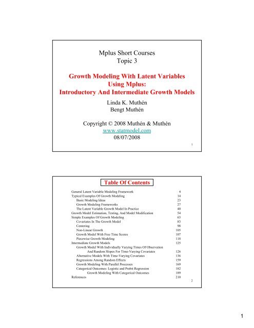
Mplus Short CoursesTopic 3Growth Modeling With Latent VariablesUsing Mplus:Introductory And Intermediate Growth ModelsLinda K. MuthénBengt MuthénCopyright © 2008 Muthén & Muthénwww.statmodel.com08/07/20081Table Of ContentsGeneral Latent Variable Modeling FrameworkTypical Examples Of Growth ModelingBasic Modeling IdeasGrowth Modeling FrameworksThe Latent Variable Growth Model In PracticeGrowth Model Estimation, Testing, And Model ModificationSimple Examples Of Growth ModelingCovariates In The Growth ModelCenteringNon-Linear GrowthGrowth Model With Free Time ScoresPiecewise Growth ModelingIntermediate Growth ModelsGrowth Model With Individually Varying Times Of ObservationAnd Random Slopes For Time-Varying CovariatesAlternative Models With Time-Varying CovariatesRegressions Among Random EffectsGrowth Modeling With Parallel ProcessesCategorical Outcomes: Logistic and Probit RegressionGrowth Modeling With Categorical OutcomesReferences4142327405463839810510711812512613615916918218921021

Mplus Background• Inefficient dissemination of statistical methods:– Many good methods contributions from biostatistics,psychometrics, etc are underutilized in practice• Fragmented presentation of methods:– Technical descriptions in many different journals– Many different pieces of limited software• Mplus: Integration of methods in one framework– Easy to use: Simple, non-technical language, graphics– Powerful: General modeling capabilities• Mplus versions– V1: November 1998– V3: March 2004– V5: November 2007– V2: February 2001– V4: February 2006• Mplus team: Linda & Bengt Muthén, Thuy Nguyen,Tihomir Asparouhov, Michelle Conn, Jean Maninger3Statistical Analysis With Latent VariablesA General Modeling FrameworkStatistical Concepts Captured By Latent VariablesContinuous Latent Variables• Measurement errors• Factors• Random effects• Frailties, liabilities• Variance components• Missing dataCategorical Latent Variables• Latent classes• Clusters• Finite mixtures• Missing data42

Statistical Analysis With Latent VariablesA General Modeling Framework (Continued)Models That Use Latent VariablesContinuous Latent Variables• Factor analysis models• Structural equation models• Growth curve models• Multilevel modelsCategorical Latent Variables• Latent class models• Mixture models• Discrete-time survival models• Missing data modelsMplus integrates the statistical concepts captured bylatent variables into a general modeling framework thatincludes not only all of the models listed above but alsocombinations and extensions of these models.5General Latent Variable Modeling Framework• Observed variablesx background variables (no model structure)y continuous and censored outcome variablesu categorical (dichotomous, ordinal, nominal) andcount outcome variables• Latent variablesf continuous variablesc– interactions among f’scategorical variables– multiple c’s63

General Latent Variable Modeling Framework7General Latent Variable Modeling Framework84

General Latent Variable Modeling Framework9General Latent Variable Modeling Framework• Observed variablesx background variables (no model structure)y continuous and censored outcome variablesu categorical (dichotomous, ordinal, nominal) andcount outcome variables• Latent variablesf continuous variablesc– interactions among f’scategorical variables– multiple c’s105

Several programs in one• Exploratory factor analysis• Structural equation modeling• Item response theory analysis• Latent class analysis• Latent transition analysis• Survival analysis• Growth modeling• Multilevel analysis• Complex survey data analysis• Monte Carlo simulationMplusFully integrated in the general latent variable framework11Overview Of Mplus Courses• Topic 1. March 18, 2008, Johns Hopkins University:Introductory - advanced factor analysis and structural equationmodeling with continuous outcomes• Topic 2. March 19, 2008, Johns Hopkins University:Introductory - advanced regression analysis, IRT, factoranalysis and structural equation modeling with categorical,censored, and count outcomes• Topic 3. August 21, 2008, Johns Hopkins University:Introductory and intermediate growth modeling• Topic 4. August 22, 2008, Johns Hopkins University:Advanced growth modeling, survival analysis, and missingdata analysis126

Overview Of Mplus Courses (Continued)• Topic 5. November 10, 2008, University of Michigan, AnnArbor: Categorical latent variable modeling with crosssectionaldata• Topic 6. November 11, 2008, University of Michigan, AnnArbor: Categorical latent variable modeling with longitudinaldata• Topic 7. March 17, 2009, Johns Hopkins University:Multilevel modeling of cross-sectional data• Topic 8. March 18, 2009, Johns Hopkins University:Multilevel modeling of longitudinal data13Typical Examples Of Growth Modeling147

LSAY DataLongitudinal Study of American Youth (LSAY)• Two cohorts measured each year beginning in 1987– Cohort 1 - Grades 10, 11, and 12– Cohort 2 - Grades 7, 8, 9, 10, 11, and 12• Each cohort contains approximately 60 schools withapproximately 60 students per school• Variables - math and science achievement items, math andscience attitude measures, and background variables fromparents, teachers, and school principals• Approximately 60 items per test with partial item overlap acrossgrades - adaptive tests15Math Total Score666462Average Score605856Male YoungerFemale YoungerMale OlderFemale Older5452507 8 9 10 11 12Grade168

Mean CurveMath Achievement40 50 60 70 807 8 9 10GradeIndividual CurvesMath Achievement40 50 60 70 807 8 9 10Grade17Sample Means for MathMath Achievement40 50 60 70 807 8 9 10GradeSample Means for Attitude Towards MathMath Attitude10 11 12 13 14 157 8 9 10Grade189

Maternal Health Project DataMaternal Health Project (MHP)• Mothers who drank at least three drinks a week duringtheir first trimester plus a random sample of mothers whoused alcohol less often• Mothers measured at fourth month and seventh month ofpregnancy, at delivery, and at 8, 18, and 36 monthspostpartum• Offspring measured at 0, 8, 18 and 36 months• Variables for mothers - demographic, lifestyle, currentenvironment, medical history, maternal psychologicalstatus, alcohol use, tobacco use, marijuana use, other illicitdrug use• Variables for offspring - head circumference, height,weight, gestational age, gender, and ethnicity19MHP: Offspring Head Circumference500Child’s Head Circumference (in millimeters)450400350300Exposed to Prenatal AlcoholAverage for All Children0 8 18 36Child’s Age (in months)2010

Loneliness In TwinsAge range: 13-854 occasions: 1991, 1995,1997, 2000, 2002/3Boomsma, D.I., Cacioppo, J.T., Muthen, B., Asparouhov, T., & Clark, S.(2007). Longitudinal Genetic Analysis for Loneliness in Dutch Twins.Twin Research and Human Genetics, 10, 267-273.21Loneliness In TwinsMalesFemalesI feel lonelyNobody loves me2211

Basic Modeling Ideas23Longitudinal Data: Three ApproachesThree modeling approaches for the regression of outcome on time(n is sample size, T is number of timepoints):• Use all n x T data points to do a single regression analysis:Gives an intercept and a slope estimate for all individuals - doesnot account for individual differences or lack of independenceof observations• Use each individual’s T data points to do n regressionanalyses: Gives an intercept and a slope estimate for eachindividual. Accounts for individual differences, but does notaccount for similarities among individuals• Use all n x T data points to do a single random effectregression analysis: Gives an intercept and a slope estimate foreach individual. Accounts for similarities among individuals bystipulating that all individuals’ random effects come from asingle, common population and models the non-independence ofobservations as show on the next page2412

Individual Development Over Time(1) y ti = η 0i + η 1i x t + ε ti(2a) η 0i(2b) η 1i= α 0 + γ 0 w i + ζ 0i= α 1 + γ 1 w i + ζ 1it = timepointy = outcomeη 0 = intercepti = individualx = time scoreη 1 = slopew = time-invariant covariateη 0yi = 1η 1wi = 2i = 3xw25Individual Development Over Timeyi = 1i = 2i = 3t = 1 t = 2 t = 3 t = 4ε 1ε 2ε 3ε 4y 1y 2y 3y 4xη 0η 1(1) y ti = η 0i + η 1i x t + ε ti(2a)(2b)η 0i = α 0 + γ 0 w i + ζ 0iη 1i = α 1 + γ 1 w i + ζ 1iw2613

Growth Modeling Frameworks27Growth Modeling Frameworks/SoftwareMultilevel(HLM)Mixed Linear(SAS PROC Mixed)SEMLatent Variable Modeling (Mplus)2814

Comparison Summary Of Multilevel,Mixed Linear, And SEM Growth Models• Multilevel and mixed linear models are the same• SEM differs from the multilevel and mixed linear models in twoways• Treatment of time scores• Time scores are data for multilevel and mixed linearmodels -- individuals can have different times ofmeasurement• Time scores are parameters for SEM growth models --time scores can be estimated• Treatment of time-varying covariates• Time-varying covariates have random effect coefficientsfor multilevel and mixed linear models -- coefficientsvary over individuals• Time-varying covariates have fixed effect coefficientsfor SEM growth models -- coefficients vary over time29Random Effects: MultilevelAnd Mixed Linear ModelingIndividual i (i = 1, 2, …, n) observed at time point t (t = 1, 2, … T).Multilevel model with two levels (e.g. Raudenbush & Bryk,2002, HLM).• Level 1: y ti = η 0i + η 1i x ti + κ i w ti + ε ti (39)• Level 2: η 0i = α 0 + γ 0 w i + ζ 0i (40)η 1i = α 1 + γ 1 w i + ζ 1i (41)κ i = α + γ w i + ζ i (42)3015

Random Effects: MultilevelAnd Mixed Linear Modeling (Continued)Mixed linear model:y ti = fixed part + random part (43)= α 0 + γ 0 w i + (α 1 + γ 1 w i ) x ti +(α + γ w i ) w ti (44)+ ζ 0i + ζ 1i x ti + ζ i w ti + ε ti . (45)E.g. “time X w i ” refers to γ 1 (e.g. Rao, 1958; Laird &Ware, 1982; Jennrich & Sluchter, 1986; Lindstrom & Bates,1988; BMDP5V; Goldstein, 2003, MLwiN; SAS PROCMIXED-Littell et al. 1996 and Singer, 1999).31Random Effects: SEM AndMultilevel ModelingSEM (Tucker, 1958; Meredith & Tisak, 1990; McArdle &Epstein 1987; SEM software):Measurement part:y ti = η 0i + η 1i x t + κ t w ti + ε ti . (46)Compare with level 1 of multilevel:y ti = η 0i + η 1i x ti + κ i w ti + ε ti . (47)Multilevel approach:• x ti as data: Flexible individually-varying times ofobservation• Slopes for time-varying covariates vary over individuals3216

Random Effects: SEM AndMultilevel Modeling (Continued)SEM approach:• x t as parameters: Flexible growth function form• Slopes for time-varying covariates vary over time pointsStructural part (same as level 2, except for κ t ):η 0i = α 0 + γ 0 w i + ζ 0i , (48)η 1i = α 1 + γ 1 w i + ζ 1i , (49)κ t not involved (parameter).33Random Effects: MixedLinear Modeling And SEMMixed linear model in matrix form:y i = (y 1i , y 2i , …, y Ti ) ́ (51)= X i α + Z i b i + e i . (52)Here, X, Z are design matrices with known values, α containsfixed effects, and b contains random effects. Compare with(43) - (45).3417

Random Effects: Mixed LinearModeling And SEM (Continued)SEM in matrix form:y i = v + Λη i + Κ x i + ε i , (53)η i = α + Βη i + Γ x i + ζ i . (54)y i = fixed part + random part= v + Λ (Ι – Β) -1 α + Λ (Ι – Β) -1 Γ x i + Κ x i+ Λ (Ι – Β) -1 ζ i + ε i .Assume x ti = x t , κ i = κ t in (39). Then (39) is handled by(53) and (40) – (41) are handled by (54), putting x t in Λ andw ti , w i in x i .Need for Λ i , Κ i , Β i , Γ i .35Growth Modeling Approached In Two Ways:Data Arranged As Wide Versus Long• Wide: Multivariate, Single-Level Approachyy ti = i i + s ix timeti + ε tiisi i regressed on w is i regressed on w iw• Long: Univariate, 2-Level Approach (CLUSTER = id)WithinBetweenitimesiywsThe intercept i is called y in Mplus3618

Multilevel Modeling In ALatent Variable FrameworkIntegrating multilevel and SEM analyses (Asparouhov & Muthén,2002).Flexible combination of random effects and other latent variables:• Multilevel models with random effects (intercepts, slopes)- Individually-varying times of observation read as data- Random slopes for time-varying covariates• SEM with factors on individual and cluster levels• Models combining random effects and factors, e.g.- Cluster-level latent variable predictors with multiple indicators- Individual-level latent variable predictors with multiple indicators• Special applications- Random coefficient regression (no clustering; heteroscedasticity)- Interactions between continuous latent variables and observedvariables37Alternative Models For Longitudinal DataGrowth Curve ModelAuto-Regressive Modely1 y2 y3 y4y1 y2 y3 y4isHybrid ModelsCurran & Bollen (2001)McArdle & Hamagami (2001)Bollen & Curran (2006)3819

Advantages Of Growth ModelingIn A Latent Variable Framework• Flexible curve shape• Individually-varying times of observation• Regressions among random effects• Multiple processes• Modeling of zeroes• Multiple populations• Multiple indicators• Embedded growth models• Categorical latent variables: growth mixtures39The Latent Variable Growth Model In Practice4020

Individual Development Over Timeyi = 1i = 2i = 3t = 1 t = 2 t = 3 t = 4ε 1ε 2ε 3ε 4y 2y 3y 4xη 0η 1y 1(1) y ti = η 0i + η 1i x t + ε ti(2a) η 0i = α 0 + γ 0 w i + ζ 0iw(2b) η 1i = α 1 + γ 1 w i + ζ 1i41Linear Growth ModelSpecifying Time Scores ForLinear Growth Models• Need two latent variables to describe a linear growthmodel: Intercept and slopeOutcome1 2 3 4Time• Equidistant time scores 0 1 2 3for slope: 0 .1 .2 .3or4221

Specifying Time Scores ForLinear Growth Models (Continued)Outcome1 2 3 4 5 6 7Time• Nonequidistant time scores 0 1 4 5 6for slope: 0 .1 .4 .5 .6or43Interpretation Of The Linear Growth FactorsModel:y ti = η 0i + η 1i x t + ε ti , (17)where in the example t = 1, 2, 3, 4 and x t = 0, 1, 2, 3:y 1i = η 0i + η 1i 0 + ε 1i , (18)η 0i = y 1i – ε 1i , (19)y 2i = η 0i + η 1i 1 + ε 2i , (20)y 3i = η 0i + η 1i 2 + ε 3i , (21)y 4i = η 0i + η 1i 3 + ε 4i . (22)4422

Interpretation Of The Linear Growth Factors(Continued)Interpretation of the intercept growth factorη 0i (initial status, level):Systematic part of the variation in the outcome variable atthe time point where the time score is zero.• Unit factor loadingsInterpretation of the slope growth factorη 1i (growth rate, trend):Systematic part of the increase in the outcome variable for atime score increase of one unit.• Time scores determined by the growth curve shape45Interpreting Growth Model Parameters• Intercept Growth Factor Parameters• Mean• Average of the outcome over individuals at thetimepoint with the time score of zero;• When the first time score is zero, it is the interceptof the average growth curve, also called initial status• Variance• Variance of the outcome over individuals at thetimepoint with the time score of zero, excluding theresidual variance4623

Interpreting Growth ModelParameters (Continued)• Linear Slope Growth Factor Parameters• Mean – average growth rate over individuals• Variance – variance of the growth rate over individuals• Covariance with Intercept – relationship betweenindividual intercept and slope values• Outcome Parameters• Intercepts – not estimated in the growth model – fixedat zero to represent measurement invariance• Residual Variances – time-specific and measurementerror variation• Residual Covariances – relationships between timespecificand measurement error sources of variationacross time47Latent Growth Model ParametersAnd Sources Of Model Misfitε 1 ε 2 ε 3 ε 4y 1 y 2 y 3 y 4η 0 η 14824

Latent Growth Model ParametersFor Four Time PointsLinear growth over four time points, no covariates.Free parameters in the H 1 unrestricted model:• 4 means and 10 variances-covariancesFree parameters in the H 0 growth model:(9 parameters, 5 d.f.):• Means of intercept and slope growth factors• Variances of intercept and slope growth factors• Covariance of intercept and slope growth factors• Residual variances for outcomesFixed parameters in the H 0 growth model:• Intercepts of outcomes at zero• Loadings for intercept growth factor at one• Loadings for slope growth factor at time scores• Residual covariances for outcomes at zero49Latent Growth Model Sources Of MisfitSources of misfit:• Time scores for slope growth factor• Residual covariances for outcomes• Outcome variable intercepts• Loadings for intercept growth factorModel modifications:• Recommended– Time scores for slope growth factor– Residual covariances for outcomes• Not recommended– Outcome variable intercepts– Loadings for intercept growth factor5025

Latent Growth Model ParametersFor Three Time PointsLinear growth over three time points, no covariates.Free parameters in the H 1 unrestricted model:• 3 means and 6 variances-covariancesFree parameters in the H 0 growth model(8 parameters, 1 d.f.)• Means of intercept and slope growth factors• Variances of intercept and slope growth factors• Covariance of intercept and slope growth factors• Residual variances for outcomesFixed parameters in the H 0 growth model:• Intercepts of outcomes at zero• Loadings for intercept growth factor at one• Loadings for slope growth factor at time scores• Residual covariances for outcomes at zero51Growth Model Means And Variancesy ti = η 0i + η 1i x t + ε ti ,x t = 0, 1, …, T – 1.Expectation (mean; E) and variance (V):E(y ti)E (y ti ) = E (η 0i ) + E (η 1i ) x t ,V (y ti ) = V (η 0i ) + V (η 1i ) x t+ 2x t Cov (η 0i , η 1i ) + V (ε ti )2V(y ti)} E(η 1i)} V(η 1i)} E(η 0i } ) V(η 0i )0 1 2 3 4t0 1 2 3 4V(ε ti ) constant over tCov(η 0 , η 1 ) = 0t5226

Growth Model Covariancesy ti= η 0i+ η 1ix t+ ε ti,x t= 0, 1, …, T –1.Cov(y ti,y t í) = V(η 0i) + V(η 1i) x tx t ́+ Cov(η 0i, η 1i) (x t+ x t ́)+ Cov(ε ti, ε t í).V(η 0t) :V(η 1i) x tx t:ttttη 0η 1η 0η 1Cov(η 0i, η 1i) x t:Cov(η 0i, η 1i) x t:ttttη 0η 1η 0η 153Growth Model Estimation, Testing, AndModel Modification5427

Growth Model Estimation, Testing, AndModel Modification• Estimation: Model parameters– Maximum-likelihood (ML) estimation under normality– ML and non-normality robust s.e.’s– Quasi-ML (MUML): clustered data (multilevel)– WLS: categorical outcomes– ML-EM: missing data, mixtures• Model Testing– Likelihood-ratio chi-square testing; robust chi square– Root mean square of approximation (RMSEA):Close fit (≤ .05)• Model Modification– Expected drop in chi-square, EPC• Estimation: Individual growth factor values (factor scores)– Regression method – Bayes modal – Empirical Bayes– Factor determinacy55CFA Modeling Estimation And TestingEstimatorsIn CFA, a covariance matrix and a mean vector are analyzed.• ML – minimizes the differences between matrix summaries(determinant and trace) of observed and estimatedvariances/covariances• Robust ML – same estimates as ML, standard errors and chisquarerobust to non-normality of outcomes and nonindependenceof observations (MLM, MLR)Chi-square test of model fitTests that the model does not fit significantly worsethan a model where the variables correlate freely – p-valuesgreater than or equal to .05 indicate good fitH 0 : Factor modelH 1 : Free variance-covariance modelIf p < .05, H 0 is rejectedNote: We want large p5628

CFA Modeling Estimation And Testing(Continued)Model fit indices (cutoff recommendations for good fit basedon Yu, 2002 / Hu & Bentler, 1999; see also Marsh et al,2004)• CFI – chi-square comparisons of the target model to thebaseline model – greater than or equal to .96/.95• TLI – chi-square comparisons of the target model to thebaseline model – greater than or equal to .95/.95• RMSEA – function of chi-square, test of close fit – less thanor equal to .05 (not good at n=100)/.06• SRMR – average correlation residuals – less than or equal to.07 (not good with binary outcomes)/.08• WRMR – average weighted residuals – less than or equal to1.00 (also good with non-normal and categorical outcomes –not good with growth models with many timepoints ormultiple group models)57Degrees Of Freedom For Chi-SquareTesting Against An Unrestricted ModelThe p value of the χ 2 test gives the probability of obtaining a χ 2value this large or larger if the H 0 model is correct (we want highp values).Degrees of Freedom:(Number of parameters in H 1 ) – (number parameters in H 0 )Number of H 1 parameters with an unrestricted Σ: p (p + 1)/2Number of H 1 parameters with unrestricted μ and Σ:p + p (p + 1)/2A degrees of freedom example – EFA• p (p + 1)/2 – (p m + m (m + 1)/2 + p – m 2 )Example: if p = 5 and m = 2, then df = 15829

Chi-Square Difference TestingOf Nested Models• When a model H a imposes restrictions on parameters ofmodel H b , H a is said to be nested within H b• To test if the nested model H a fits significantly worse than H b ,a chi-square test can be obtained as the difference in the chisquarevalues for the two models (testing against anunrestricted model) using as degrees of freedom thedifference in number of parameters for the two models• The chi-square difference is the same as 2 times thedifference in log likelihood values for the two models• The chi-square theory does not hold if H a has restricted any ofthe H b parameters to be on the border of their admissibleparameter space (e.g. variance = 0)59CFA Model ModificationModel modification indices are estimated for all parameters thatare fixed or constrained to be equal.• Modification Indices – expected drop in chi-square if theparameter is estimated• Expected Parameter Change Indices – expected value of theparameter if it is estimated• Standardized Expected Parameter Change Indices –standardized expected value of the parameter if it is estimatedModel Modifications• Residual covariances• Factor cross loadings6030

Alternative Growth Model ParameterizationsParameterization 1 – for continuous outcomesy ti = 0 + η 0i + η 1i x t + ε ti , (32)η 0i = α 0 + ζ 0i , (33)η 1i = α 1 + ζ 1i . (34)Parameterization 2 – for categorical outcomes andmultiple indicatorsy ti = v + η 0i + η 1i x t + ε ti , (35)η 0i = 0 + ζ 0i , (36)η 1i = α 1 + ζ 1i . (37)61Alternative Growth Model ParameterizationsParameterization 1 – for continuous outcomes• Outcome variable intercepts fixed at zero• Growth factor means free to be estimatedMODEL:i BY y1-y4@1;s BY y1@0 y2@1 y3@2 y4@3;[y1-y4@0 i s];Parameterization 2 – for categorical outcomes andmultiple indicators• Outcome variable intercepts constrained to be equal• Intercept growth factor mean fixed at zeroMODEL:i BY y1-y4@1;s BY y1@0 y2@1 y3@2 y4@3;[y1-y4] (1);[i@0 s];6231

Simple Examples Of Growth Modeling63Steps In Growth Modeling• Preliminary descriptive studies of the data: means,variances, correlations, univariate and bivariatedistributions, outliers, etc.• Determine the shape of the growth curve from theoryand/or data• Individual plots• Mean plot• Consider change in variance across time• Fit model without covariates using fixed time scores• Modify model as needed• Add covariates6432

LSAY Math AchievementMean CurveMath Achievement40 50 60 70 807 8 9 10GradeIndividual CurvesMath Achievement40 50 60 70 807 8 9 10Grade65TITLE:DATA:!!Input For LSAY TYPE=BASIC AnalysisVARIABLE:!lsayid =!schcode =!mothed =!Student id7 th grade school codemother’s education(1=LT HS diploma, 2=HS diploma, 3=Some college,!4=4yr college degree, 5=advanced degree)!homeres = Home math and science resources!mthcrs7-mthcrs12 = Highest math course taken during each grade!(0 = no course, 1 – low,basic, 2 = average, 3 = high,ANALYSIS:PLOT:Basic runFILE = lsayfull_dropout.dat;NAMES = lsayid schcode female mothed homeres math7math8 math9 math10 math11 math12mthcrs7 mthcrs8 mthcrs9 mthcrs10 mthcrs11 mthcrs12;4 = pre-algebra, 5 = algebra I, 6 = geometry,7 = algebra II, 8 = pre-calc, 9 = calculus)TYPE = BASIC;TYPE = PLOT3;SERIES = math7-math10(*);6633

Sample Statistics For LSAY DataMeansCovariancesMATH7MATH8MATH9MATH10MATH750.356MATH7103.86893.096104.328110.003n = 3102MATH853.872MATH8121.294121.439125.355MATH957.962MATH9161.394157.656MATH1062.250MATH10189.096CorrelationsMATH7MATH8MATH9MATH10MATH71.0000.8290.8060.785MATH81.0000.8680.828MATH91.0000.902MATH101.00067math7 math8 math9 math10is6834

TITLE:DATA:VARIABLE:MODEL:Input For LSAY Linear Growth ModelWithout CovariatesGrowth 7 – 10, no covariatesFILE = lsayfull_dropout.dat;NAMES = lsayid schcode female mothed homeresmath7 math8 math9 math10 math11 math12mthcrs7 mthcrs8 mthcrs9 mthcrs10 mthcrs11 mthcrs12;USEV = math7-math10;MISSING = ALL(9999);i BY math7-math10@1;s BY math7@0 math8@1 math9@2 math10@3;[math7-math10@0];[i s];OUTPUT: SAMPSTAT STANDARDIZED RESIDUAL MODINDICES (3.84);Alternative language:MODEL: i s | math7@0 math8@1 math9@2 math10@3;69Output Excerpts LSAY Linear GrowthModel Without Covariates (Continued)Model ResultsIBYMATH7MATH8MATH9MATH10SBYMATH7MATH8MATH9MATH10Estimates S.E. Est./S.E. Two-TailedP-Value1.0001.0001.0001.0000.0001.0002.0003.0000.0000.0000.0000.0000.0000.0000.0000.000999.000999.000999.000999.000999.000999.000999.000999.000999.000999.000999.000999.000999.000999.000999.000999.0007035

Output Excerpts LSAY Linear GrowthModel Without Covariates (Continued)MeansISInterceptsMATH7MATH8MATH9MATH10Estimates50.2023.9390.0000.0000.0000.000S.E.0.1800.0590.0000.0000.0000.000Est./S.E.279.52366.460999.000999.000999.000999.000Two-tailedP-value0.0000.000999.000999.000999.000999.00071Output Excerpts LSAY Linear GrowthModel Without Covariates (Continued)Residual VariancesMATH7MATH8MATH9MATH10VariancesISI WITHSR-SquareObservedVariableEstimates17.43018.44016.18417.21986.1594.7928.031R-SquareS.E.1.0020.7500.7571.3012.6060.2950.654Est./S.E.17.40024.59620.56113.23033.06716.26212.276Two-tailedP-value0.0000.0000.0000.0000.0000.0000.000MATH7MATH8MATH9MATH100.8320.8530.8950.9127236

Output Excerpts LSAY Linear GrowthModel Without Covariates (Continued)Tests Of Model FitChi-Square Test of Model FitValue 86.541Degrees of Freedom 5P-Value 0.0000CFI/TLICFI 0.992TLI 0.990RMSEA (Root Mean Square Error Of Approximation)Estimate 0.07390 Percent C.I. 0.060 0.086Probability RMSEA

Output Excerpts LSAY Linear GrowthModel Without Covariates (Continued)Modification IndicesM.I.E.P.C.Std.E.P.C.StdYX E.P.C.Means/Intercepts/Thresholds[ MATH7 ]18.0110.6710.6710.066[ MATH8 ]12.506-0.362-.362-0.03275Linear Growth Model Without Covariates:Adding Correlated Residualsmath7 math8 math9 math10isMODEL:i s | math7@0 math8@1 math9@2 math10@3;math7-math9 PWITH math8-math10;7638

Output Excerpts LSAY Linear Growth ModelWithout Covariates:Adding Correlated ResidualsTests Of Model FitChi-Square Test of Model FitValue 18.519Degrees of Freedom 2P-Value 0.0000CFI/TLICFI 0.998TLI 0.995RMSEA (Root Mean Square Error Of Approximation)Estimate 0.05290 Percent C.I. 0.032 0.074Probability RMSEA

Output Excerpts LSAY:Adding Correlated Residuals (Continued)VariancesEstimatesS.E.Est./S.E.Two-tailedP-valueI92.0384.16722.0850.000S3.0430.7893.8580.000Residual VariancesMATH711.8713.4663.4250.001MATH814.0271.9807.0850.000MATH932.5962.60912.4920.000MATH1033.8574.8157.0320.00079Output Excerpts LSAY:Adding Correlated Residuals (Continued)ESTIMATED MODEL AND RESIDUALS (OBSERVED – ESTIMATED)Model Estimated Means/Intercepts/ThresholdsMATH7MATH8MATH9MATH10150.203 54.140 58.07662.012Residuals for Means/Intercepts/ThresholdsMATH7MATH8MATH9MATH1010.153 -0.267 -0.1140.238Standardized Residuals (z-scores) forMeans/Intercepts/ThresholdsMATH7MATH8MATH9MATH1014.198 -4.109 -1.2565.199Normalized Residuals for Means/Intercepts/ThresholdsMATH7MATH8MATH9MATH1010.834-1.317-0.4780.9048040

Output Excerpts LSAY:Adding Correlated Residuals (Continued)Model Estimated Covariances/Correlations/ResidualCorrelationsMATH7MATH8MATH9MATH7MATH8MATH9MATH10MATH7103.91093.093104.304-0.0410.0020.024-0.434121.375121.441MATH10110.437 125.700 158.025 190.083Residuals for Covariances/Correlations/Residual CorrelationsMATH7MATH8MATH8-0.081-0.002-0.345MATH9161.339MATH90.055-0.368MATH10MATH10-0.98781Output Excerpts LSAY:Adding Correlated Residuals (Continued)Standardized Residuals (z-scores) forCovariances/Correlations/Residual CorrMATH7MATH8MATH9MATH10Normalized Residuals for Covariances/Correlations/ResidualCorrelationsMATH7MATH8MATH9 MATH10MATH7MATH8MATH9MATH10MATH7999.000999.0000.279999.000-0.0160.0010.008-0.130MATH8999.000999.000999.000-0.025-0.001-0.092MATH90.297999.0000.012-0.081MATH10999.000-0.1858241

Covariates In The Growth Model83Covariates In The Growth Model• Types of covariates• Time-invariant covariates—vary across individuals nottime, explain the variation in the growth factors• Time-varying covariates—vary across individuals andtime, explain the variation in the outcomes beyond thegrowth factors8442

Time-Invariant AndTime-Varying Covariatesy 1 y 2 y 3 y 4η 0η 1w a 21a 22a 23a 2485LSAY Growth Model WithTime-Invariant Covariatesmath7 math8 math9 math10ismothedhomeres8643

Input Excerpts For LSAY Linear GrowthModel With Time-Invariant CovariatesTITLE:DATA:VARIABLE:ANALYSIS:MODEL:Growth 7 – 10, no covariatesFILE = lsayfull_dropout.dat;NAMES = lsayid schcode female mothed homeresmath7 math8 math9 math10 math11 math12mthcrs7 mthcrs8 mthcrs9 mthcrs10 mthcrs11 mthcrs12;MISSING = ALL (999);USEVAR = math7-math10 mothed homeres;!ESTIMATOR = MLR;i s | math7@0 math8@1 math9@2 math10@3;i s ON mothed homeres;Alternative language:MODEL:i BY math7-math10@1;s BY math7@0 math8@1 math9@2 math10@3;[math7-math10@0];[i s];i s ON mothed homeres;87Output Excerpts LSAY Growth ModelWith Time-Invariant CovariatesTests Of Model Fit for MLn = 3116Chi-Square Test of Model FitValueDegrees of FreedomP-ValueCFI/TLICFITLIRMSEA (Root Mean Square Error Of Approximation)Estimate90 Percent C.I.Probability RMSEA

Output Excerpts LSAY Growth ModelWith Time-Invariant Covariates (Continued)Tests Of Model Fit for MLRChi-Square Test of Model FitValueDegrees of FreedomP-ValueScaling Correction Factorfor MLRCFI/TLICFITLIRMSEA (Root Mean Square Error Of Approximation)Estimate90 Percent C.I.Probability RMSEA

Output Excerpts LSAY Growth ModelWith Time-Invariant Covariates (Continued)EstimateS.E.Est./S.E.Two-TailedP-ValueSWITHI4.131Residual Variances1.2443.3200.001I71.8883.63019.8040.000S3.3130.7244.5790.000InterceptsIS38.4342.6360.4970.18177.39114.5610.0000.00091Output Excerpts LSAY Growth ModelWith Time-Invariant Covariates (Continued)R-SquareObservedVariableMATH7MATH8MATH9MATH10LatentVariableISR-Square0.8760.8630.8170.854R-Square.204.0919246

Output Excerpts LSAY Growth ModelWith Time-Invariant Covariates (Continued)TECHNICAL 4 OUTPUTESTIMATES DERIVED FROM THE MODELESTIMATED MEANS FOR THE LATENT VARIABLESISFEMALEMOTHEDHOMERES50.2193.9440.4782.3473.11893Output Excerpts LSAY Growth ModelWith Time-Invariant Covariates (Continued)ISFEMALEMOTHEDHOMERESISFEMALEMOTHEDHOMERESESTIMATED COVARIANCE MATRIX FOR THE LATENT VARIABLESI90.2646.4110.3503.2265.901IS3.647-0.0580.3730.891SFEMALE0.250-0.024-0.071FEMALEMOTHED1.0880.467ESTIMATED CORRELATION MATRIX FOR THE LATENT VARIABLES1.0000.3530.0740.3260.3681.000-0.0610.1870.2761.000-0.047-0.084MOTHED1.0000.265HOMERES2.853HOMERES1.0009447

Model Estimated Average And IndividualGrowth Curves With CovariatesModel:y ti = η 0i + η 1i x t + ε ti , (23)η 0i = α 0 + γ 0 w i + ζ 0i , (24)η 1i = α 1 + γ 1 w i + ζ 1i , (25)Estimated growth factor means:Ê(η 0i ) = ˆ α0+ˆ0w γ , (26)Ê(η 1i ) = ˆ α + γ . (27)1ˆ1 wEstimated outcome means:Ê(y ti ) = Ê(η 0i ) + Ê(η 1i ) x t . (28)Estimated outcomes for individual i :yˆ ti = ηˆ0i + ηˆ1i xtwhere ˆ0iη and ηˆ1 i are estimated factor scores. y ti can beused for prediction purposes.(29)95Model Estimated Means With CovariatesModel estimated means are available using the TECH4 and RESIDUAL options ofthe OUTPUT command.Estimated Intercept Mean = Estimated Intercept +Estimated Slope (Female)*Sample Mean (Female) +Estimated Slope (Mothed)*Sample Mean (Mothed) +Estimated Slope (Homeres)*Sample Mean (Homeres)38.43 + 2.12*0.48 + 2.26*2.35 + 1.75*3.12 = 50.22Estimated Slope Mean = Estimated Intercept +Estimated Slope (Female)*Sample Mean (Female) +Estimated Slope (Mothed)*Sample Mean (Mothed) +Estimated Slope (Homeres)*Sample Mean (Homeres)2.64 – 0.13*0.48 + 0.22*2.35 + 0.27*3.11 = 3.949648

Centering• Centering determines the interpretation of the interceptgrowth factor• The centering point is the timepoint at which the time score iszero• A model can be estimated for different centering pointsdepending on which interpretation is of interest• Models with different centering points give the same modelfit because they are reparameterizations of the model• Changing the centering point in a linear growth model withfour timepointsTimepoints 1 2 3 4Centering atTime scores 0 1 2 3 Timepoint 1-1 0 1 2 Timepoint 2-2 -1 0 1 Timepoint 3-3 -2 -1 0 Timepoint 499Input Excerpts For LSAY Growth ModelWith Covariates Centered At Grade 10MODEL:OUTPUT:i s | math7@-3 math8@-2 math9@-1 math10@0;i s ON female mothed homeres;math7-math9 PWITH math8-math10;TECH1 RESIDUAL STANDARDIZED MODINDICES TECH4;Alternative language:MODEL:i BY math7-math10@1;s BY math7@-3 math8@-2 math9@-1 math10@0;[math7-math10@0];[i s];i s ON female mothed homeres;10050

Output Excerpts LSAY Growth ModelWith Covariates Centered At Grade 10Tests of Model FitCHI-SQUARE TEST OF MODEL FITn = 3116Value 33.611Degrees of Freedom 8P-Value 0.000RMSEA (ROOT MEAN SQUARE ERROR OF APPROXIMATION)Estimate .03290 Percent C.I. .021 .044Probability RMSEA

Further Readings On Introductory Growth ModelingBijleveld, C. C. J. H., & van der Kamp, T. (1998). Longitudinal dataanalysis: Designs, models, and methods. Newbury Park: Sage.Bollen, K.A. & Curran, P.J. (2006). Latent curve models. A structuralequation perspective. New York: Wiley.Duncan, T., Duncan S. & Strycker, L. (2006). An introduction to latentvariable growth curve modeling. Second edition. LawrenceErlbaum: New York.Muthén, B. & Khoo, S.T. (1998). Longitudinal studies of achievementgrowth using latent variable modeling. Learning and IndividualDifferences, Special issue: latent growth curve analysis, 10, 73-101. (#80)Muthén, B. & Muthén, L. (2000). The development of heavy drinkingand alcohol-related problems from ages 18 to 37 in a U.S. nationalsample. Journal of Studies on Alcohol, 61, 290-300. (#83)103Further Readings On Introductory Growth Modeling(Continued)Raudenbush, S.W. & Bryk, A.S. (2002). Hierarchical linear models:Applications and data analysis methods. Second edition. NewburyPark, CA: Sage Publications.Singer, J.D. & Willett, J.B. (2003). Applied longitudinal data analysis.Modeling change and event occurrence. New York, NY: OxfordUniversity Press.Snijders, T. & Bosker, R. (1999). Multilevel analysis. An introductionto basic and advanced multilevel modeling. Thousand Oakes, CA:Sage Publications.10452

Non-Linear Growth105Six Ways To Model Non-Linear Growth• Estimated time scores• Quadratic (cubic) growth model• Fixed non-linear time scores• Piecewise growth modeling• Time-varying covariates• Non-linearity of random effects10653

Growth Model With Free Time Scores107Specifying Time Scores For Non-LinearGrowth Models With Estimated Time ScoresNon-linear growth models with estimated time scores• Need two latent variables to describe a non-linear growthmodel: Intercept and slopeOutcome∗∗Outcome∗∗1 2 3 4Time1 2 3 4TimeTime scores: 0 1 Estimated Estimated10854

Interpretation Of Slope Growth Factor MeanFor Non-Linear Models• The slope growth factor mean is the expected change in theoutcome variable for a one unit change in the time score• In non-linear growth models, the time scores should bechosen so that a one unit change occurs betweentimepoints of substantive interest.• An example of 4 timepoints representing grades 7, 8, 9,and 10• Time scores of 0 1 * * – slope factor mean refers toexpected change between grades 7 and 8• Time scores of 0 * * 1 – slope factor mean refers toexpected change between grades 7 and 10109Growth Model With Free Time Scores• Identification of the model – for a model with two growthfactors, at least one time score must be fixed to a non-zerovalue (usually one) in addition to the time score that isfixed at zero (centering point)• Interpretation—cannot interpret the mean of the slopegrowth factor as a constant rate of change over alltimepoints, but as the rate of change for a time scorechange of one.• Approach—fix the time score following the centering pointat one11055

Input Excerpts For LSAYLinear Growth Model With Free Time ScoresWithout CovariatesMODEL:i s | math7@0 math8@1 math9@2 math10@3 math11@4math12*5;Alternative language:MODEL:i BY math7-math12@1;s BY math7@0 math8@1 math9@2 math10@3 math11@4math12*5;[math7-math12@0];[i s];111Output Excerpts LSAY Growth ModelWith Free Time Scores Without CovariatesTests Of Model Fitn = 3102Chi-Square Test of Model FitValueDegrees of FreedomP-ValueCFI/TLICFITLIRMSEA (Root Mean Square Error Of Approximation)Estimate90 Percent C.I.Probability RMSEA

Output Excerpts LSAY Growth ModelWith Free Time Scores WithoutCovariates (Continued)I |MATH7MATH8MATH9MATH10MATH11MATH12S |MATH7MATH8MATH9MATH10Estimate1.0001.0001.0001.0001.0001.0000.0001.0002.0003.000S.E.0.0000.0000.0000.0000.0000.0000.0000.0000.0000.000Est./S.E.999.000999.000999.000999.000999.000999.000999.000999.000999.000999.000Two-TailedP-Value999.000999.000999.000999.000999.000999.000999.000999.000999.000999.000113Output Excerpts LSAY Growth ModelWith Free Time Scores WithoutCovariates (Continued)EstimateS.E.Est./S.E.Two-TailedP-ValueMATH114.0000.000999.000999.000MATH124.0950.04297.2360.000SWITHIVariances4.9860.7416.7250.000I91.3743.04629.9940.000S4.0010.27614.6660.000MeansIS50.3233.7520.1800.049279.61276.4720.0000.00011457

Quadratic growth modelSpecifying Time Scores ForQuadratic Growth Models2y ti = η 0i + η 1i x t + η 2i x t + ε ti ory2ti = η0i+ η1i⋅(xt− c ) + η2i⋅(xt− c )where c is a centering constant, e.g.• Need three latent variables to describe a quadratic growthmodel: Intercept, linear slope, quadratic slopexOutcome1 2 3 4Time• Linear slope time scores: 0 1 2 3 or 0 .1 .2 .3• Quadratic slope time scores: 0 1 4 9 or 0 .01 .04 .09115Specifying Time Scores For Non-LinearGrowth Models With Fixed Time ScoresNon-Linear Growth Models with Fixed Time scores• Need two latent variables to describe a non-linear growthmodel: Intercept and slopeGrowth model with a logarithmic growth curve--ln(t)Outcome1 2 3 4TimeTime scores: 0 0.69 1.10 1.3911658

Specifying Time Scores For Non-LinearGrowth Models With Fixed Time Scores (Continued)Growth model with an exponential growth curve–exp(t-1) - 1Outcome1 2 3 4TimeTime scores: 0 1.72 6.39 19.09117Piecewise Growth Modeling11859

Piecewise Growth Modeling• Can be used to represent different phases of development• Can be used to capture non-linear growth• Each piece has its own growth factor(s)• Each piece can have its own coefficients for covariates201510501 2 3 4 5 6One intercept growth factor, two slope growth factorss1: 0 1 2 2 2 2 Time scores piece 1s2: 0 0 0 1 2 3 Time scores piece 2119Piecewise Growth Modeling (Continued)201510501 2 3 4 5 6Two intercept growth factors, two slope growth factors0 1 2 Time scores piece 10 1 2 Time scores piece 2Sequential model12060

LSAY Piecewise Linear Growth Modeling:Grades 7-10 and 10-12math7 math8 math9 math10math11math121233 3 1 2i s1 s2121Input For LSAY Piecewise Growth ModelWith CovariatesMODEL:i s1 | math7@0 math8@1 math9@2 math10@3 math11@3math12@3;i s2 | math7@0 math8@0 math9@0 math10@0 math11@1math12@2;i s1 s2 ON female mothed homeres;Alternative language:MODEL:i BY math7-math12@1;s1 BY math7@0 math8@1 math9@2 math10@3 math11@3math12@3;s2 BY math7@0 math8@0 math9@0 math10@0 math11@1math12@2;[math7-math12@0];[i s1 s2];i s1 s2 ON female mothed homeres;12261

Output Excerpts LSAY Piecewise Growth ModelWith CovariatesTests of Model FitCHI-SQUARE TEST OF MODEL FITn = 3116Value 229.22Degrees of Freedom 21P-Value 0.0000RMSEA (ROOT MEAN SQUARE ERROR OF APPROXIMATION)Estimate 0.05690 Percent C.I. 0.050 0.063Probability RMSEA

Intermediate Growth Models125Growth Model With Individually-Varying TimesOf Observation And Random SlopesFor Time-Varying Covariates12663

Growth Modeling In Multilevel TermsTime point t, individual i (two-level modeling, no clustering):y ti : repeated measures of the outcome, e.g. math achievementa 1ti : time-related variable; e.g. grade 7-10a 2ti : time-varying covariate, e.g. math course takingx i : time-invariant covariate, e.g. grade 7 expectationsTwo-level analysis with individually-varying times of observation andrandom slopes for time-varying covariates:Level 1: y ti = π 0i + π 1i a 1ti + π 2ti a 2ti + e ti , (55)Level 2:π 0i = ß 00 + ß 01 x i + r 0i ,π 1i = ß 10 + ß 11 x i + r 1i , (56)π 2i = ß 20 + ß 21 x i + r 2i .127math7 math8 math9 math10isstvcfemalemothedhomerescrs7crs8 crs9 crs1012864

Input For Growth Model With IndividuallyVarying Times Of ObservationTITLE:DATA:VARIABLE:Growth model with individually varying times ofobservation and random slopesFILE IS lsaynew.dat;FORMAT IS 3F8.0 F8.4 8F8.2 3F8.0;NAMES ARE math7 math8 math9 math10 crs7 crs8 crs9crs10 female mothed homeres a7-a10;! crs7-crs10 = highest math course taken during each! grade (0=no course, 1=low, basic, 2=average, 3=high.! 4=pre-algebra, 5=algebra I, 6=geometry,! 7=algebra II, 8=pre-calc, 9=calculus)MISSING ARE ALL (9999);CENTER = GRANDMEAN (crs7-crs10 mothed homeres);TSCORES = a7-a10;129Input For Growth Model With IndividuallyVarying Times Of Observation (Continued)DEFINE:ANALYSIS:MODEL:OUTPUT:math7 = math7/10;math8 = math8/10;math9 = math9/10;math10 = math10/10;TYPE = RANDOM MISSING;ESTIMATOR = ML;MCONVERGENCE = .001;i s | math7-math10 AT a7-a10;stvc | math7 ON crs7;stvc | math8 ON crs8;stvc | math9 ON crs9;stvc | math10 ON crs10;i ON female mothed homeres;s ON female mothed homeres;stvc ON female mothed homeres;i WITH s;stvc WITH i;stvc WITH s;TECH8;13065

Output Excerpts For Growth Model WithIndividually Varying Times Of ObservationAnd Random Slopes For Time-Varying CovariatesTests of Model FitLoglikelihoodn = 2271H0 Value -8199.311Information CriteriaNumber of Free Parameters 22Akaike (AIC) 16442.623Bayesian (BIC) 16568.638Sample-Size Adjusted BIC 16498.740(n* = (n + 2) / 24)131Output Excerpts For Growth Model With IndividuallyVarying Times Of Observation And Random SlopesFor Time-Varying Covariates (Continued)Model ResultsIONFEMALEMOTHEDHOMERESSONFEMALEMOTHEDHOMERESSTVC ONFEMALEMOTHEDHOMERESIWITHSSTVC WITHISEstimates0.1870.1870.159-0.0250.0150.019-0.0080.0030.0090.0380.0110.004S.E.0.0360.0180.0110.0120.0060.0040.0130.0070.0040.0060.0050.002Est./S.E.5.24710.23114.194-2.0172.4294.835-0.5900.4292.1676.4452.0872.03313266

Output Excerpts For Growth Model With IndividuallyVarying Times Of Observation And Random SlopesFor Time-Varying Covariates (Continued)InterceptsMATH7MATH8MATH9MATH10ISSTVC0.0000.0000.0000.0004.9920.4170.1130.0000.0000.0000.0000.0250.0090.0100.0000.0000.0000.000198.45647.27511.416Residual VariancesMATH7MATH8MATH9MATH10ISSTVC0.1850.1780.1560.1690.5700.0360.0120.0110.0080.0080.0140.0230.0030.00216.46422.23218.49712.50025.08712.0645.055133Why No Chi-Square With Random SlopesFor Random Variables?Consider as an example individually-varying times of observationa 1ti :y = π + π a + eti( y | a ) = V ( π ) + V ( π ) a + 2 a Cov( π , π ) V ( e )ti0i1ti1i1ti0i21tiV +The variance of y changes as a function of a 1ti values.Not a constant Σ to test the model fit for.ti1i1ti0i1iti13467

Maximum-Likelihood AlternativesNote that [y, x] = [y | x] * [x], where the marginal distribution [x]is unrestricted.Normal theory ML for• [y, x]: Gives the same results as [y | x] when there is nomissing data (Joreskog & Goldberger, 1975). Typically used inSEM– With missing data on x, the normality assumption for x isan additional assumption than when using [y | x]• [y | x]: Makes normality assumptions for residuals, not forx. Typically used outside SEM– Used with Type = Random, Type = Mixture, and withcategorical, censored, and count outcomes– Deletes individuals with missing on any x• [y, x] versus [y | x] gives different sample sizes and thelikelihood and BIC values are not on a comparable scale135Alternative ModelsWith Time-Varying Covariates13668

Alternative ModelsWith Time-Varying CovariatesModel M1Model M2math7 math8 math9 math10math7 math8 math9 math10iissstvcfemalefemalemothedmothedhomerescrs7crs8 crs9 crs10homerescrs7crs8 crs9 crs10137Input Excerpts Model M1ANALYSIS:TYPE = RANDOM; ! gives loglikelihood in [y | x] metricMODEL:i s | math7@0 math8@1 math9@2 math10@3;i s ON female mothed homeres;math7 ON mthcrs7;math8 ON mthcrs8;math9 ON mthcrs9;math10 ON mthcrs10;13869

Output Excerpts Model M1TESTS OF MODEL FITChi-Square Test of Model FitValueDegrees of FreedomP-ValueScaling Correlation Factorfor MLR1143.173*0.0001.058* The chi-square value for MLM, MLMV, MLR, ULSMV, WLSM andWLSMV cannot be used for chi-square difference tests. MLM,MLR and WLSM chi-square difference testing is described inthe Mplus Technical Appendices at www.statmodel.com. Seechi-square difference testing in the index of the MplusUser’s Guide.23139Output Excerpts Model M1 (Continued)Chi-Square Test of Model Fit for the Baseline ModelValue8680.167Degrees of Freedom34P-Value0.000CFI/TLICFI0.870TLI0.808LoglikelihoodH0 Value-26869.760H0 Scaling Correlation Factor1.159for MLRH1 Value-26264.830H1 Scaling Correlation Factor1.104for MLR14070

Output Excerpts Model M1 (Continued)Information CriteriaNumber of Free ParametersAkaike (AIC)Bayesian (BIC)Sample-Size Adjusted BIC1953777.52053886.35153825.985(n* = (n = 2) / 24)RMSEA (Root Mean Square Error of Approximation)Estimate0.146SRMR (Standardized Root Mean Square Residual)Value0.165141Output Excerpts Model M1 (Continued)EstimateS.E.Est./S.E.Two-TailedP-ValueIONFEMALE1.8770.3575.2610.000MOTHED1.9260.2039.4970.000HOMERES1.6080.11314.1810.000SFEMALEON-0.2360.125-1.8930.058MOTHED0.1670.0662.5450.011HOMERES0.1930.0424.5560.000MATH7 ONMTHCRS71.0420.1576.6440.000MATH8ONMTHCRS80.8980.1028.7940.00014271

72143Output Excerpts Model M1 (Continued)0.00043.6210.0964.202S999.000999.0000.0000.000MATH9999.000999.0000.0000.000MATH8999.000999.0000.0000.000MATH7Intercepts0.0006.1130.6874.200ISWITH0.0008.9660.1020.911MTHCRS10MATH10ON0.00010.6380.0870.929MTHCRS9MATH9ONP-Value0.000190.1580.26350.063I999.000999.0000.0000.000MATH10Two-TailedEst./S.E.S.E.Estimate144Output Excerpts Model M1 (Continued)0.00010.5810.3593.800S0.00024.6222.39358.919I0.00010.6511.67117.795MATH100.00016.5011.01016.672MATH90.00018.5181.00218.554MATH80.00013.8951.34118.640MATH7Residual VariancesP-ValueTwo-TailedEst./S.E.S.E.Estimate

Output Excerpts Model M1 (Continued)MODIFICATION INDICESMinimum M.I. value for printing the modification index 10.000ON/BY StatementsM.I.E.P.C.MATH 7ON I/IBY MATH715.3930.014MATH7ON S/SMATH8BY MATH7ON I/16.8130.172IBY MATH811.067-0.008MATH8ON S/SBY MATH815.769-0.107SION IBY S/999.0000.000145Output Excerpts Model M1 (Continued)M.I.E.P.C.ON StatementsION MATH760.2010.718ION MATH858.5500.464ION MATH9116.4470.600ION MATH10118.9560.786ION MTHCRS7582.9705.844ION MTHCRS8373.1813.119ION MTHCRS9475.1872.540ION MTHCRS10379.5352.012SON MATH755.4440.298SON MATH9118.0640.322SON MATH1024.3550.221SON MTHCRS7203.7101.334SON MTHCRS886.1090.54314673

Output Excerpts Model M1 (Continued)M.I.E.P.C.SON MTHCRS990.5600.453SON MTHCRS10118.4780.559MATH7ON MATH715.3930.014MATH7ON MATH817.3590.013MATH7ON MATH914.8050.011MATH7ON MATH1018.9910.012MATH7ON MTHCRS848.8650.873MATH7ON MTHCRS963.4900.676MATH7ON MTHCRS1022.1600.337MATH8ON MATH811.438-0.007MATH8ON MATH1013.204-0.007MATH8ON MTHCRS782.7391.467MATH8ON MTHCRS912.7430.321147Output Excerpts Model M1 (Continued)M.I.E.P.C.MATH9ON MTHCRS726.1830.776MATH9ON MTHCRS816.0270.494MATH9ON MTHCRS1069.4800.781MATH10ON MTHCRS819.6650.629MATH10ON MTHCRS948.6780.91114874

Alternative ModelsWith Time-Varying CovariatesModelLoglikelihood# of parametersBICM1-26,8701953,886M2M3-26,846-26,463222653,86153,127n = 2271 (using [y|x] approach)M1: Fixed slopes for TICs, varying across gradeM2: Random slope for TICs, same across gradeM3: M2 + i and s regressed on TICs (see model diagram)149Time-Varying Covariates: Model M3math7 math8 math9 math10isstvcfemalemothedhomerescrs7crs8 crs9 crs1015075

Input Excerpt Model M3ANALYSIS:TYPE = RANDOM;MODEL:i s | math7@0 math8@1 math9@2 math10@3;stvc | math7 ON mthcrs7;stvc | math8 ON mthcrs8;stvc | math9 ON mthcrs9;stvc | math10 ON mthcrs10;stvc WITH i s;i s stvc ON female mothed homeres;i ON mthcrs7;s ON mthcrs8-mthcrs10;151Output Excerpts Time-Varying Covariates:Model M3EstimateS.E.Est./S.E.Two-TailedP-ValueIONFEMALE1.4440.3254.4490.000MOTHEDHOMERES1.2591.1440.1840.1046.86011.0410.0000.000MTHCRS75.0950.18827.0400.000SONFEMALE-0.3950.123-3.2150.001MOTHEDHOMERES-0.0180.0520.0640.042-0.2831.2490.7770.212MTHCRS80.0990.0611.6270.104MTHCRS90.2540.0614.1880.000MTHCRS100.3410.0536.4710.00015276

77153999.000999.0000.0000.000MATH80.4460.7620.6300.480ISWITH0.9340.0830.1850.015S0.863-0.1730.453-0.078ISTVCWITH0.0871.7100.0410.070HOMERES0.8980.1290.0660.009MOTHED0.499-0.6770.123-0.083FEMALESTVCONP-Value999.000999.0000.0000.000MATH7InterceptsTwo-TailedEst./S.E.S.E.EstimateOutput Excerpts: Model M3 (Continued)1540.0162.4100.2550.615STVC0.00010.1180.3383.423S0.00016.6900.93615.624MATH90.00018.3220.93117.061MATH80.00014.5411.30418.968MATH7Residual Variances0.0292.1880.1060.231STVC0.00045.0710.0944.257S0.000209.0850.24050.244I999.000999.0000.0000.000MATH10999.000999.0000.0000.000MATH9P-Value0.00023.7921.89144.980I0.00011.0741.49416.550MATH10Two-TailedEst./S.E.S.E.EstimateOutput Excerpts: Model M3 (Continued)

Time-Varying CovariatesRepresenting Status Changeyx155Marital Status Change And Alcohol Use(Curran, Muthen, & Harford, 1998).51 .48 .50 .41Time 1Alcohol UseTime 2Alcohol UseTime 3Alcohol UseTime 4Alcohol UseAge1.01.0 1.0Gender.31-.21AlcoholUseIntercept1.01.0 1.01.0Black.23.14.841.0 1.5* 2.5* 1.01.01.0 1.0 1.0 1.0Hispanic.11.08AlcoholUseSlopeTime 1IncrementalChangeTime 2IncrementalChangeTime 3IncrementalChangeTime 4IncrementalChangeEducation.96x 1 x 2 x-.29 -.28 -.20 -.20Time 1 Time 2 Time 3 Time 4Status Status Status Status315678

Computational Issues For Growth Models• Decreasing variances of the observed variables over time may make themodeling more difficult• Scale of observed variables – keep on a similar scale• Convergence – often related to starting values or the type of model beingestimated• Program stops because maximum number of iterations has been reached• If no negative residual variances, either increase the number ofiterations or use the preliminary parameter estimates as starting values• If there are large negative residual variances, try better starting values• Program stops before the maximum number of iterations has beenreached• Check if variables are on a similar scale• Try new starting values• Starting values – the most important parameters to give starting values to areresidual variances and the intercept growth factor mean• Convergence for models using the | symbol• Non-convergence may be caused by zero random slope variances whichindicates that the slopes should be fixed rather than random157Advantages Of Growth ModelingIn A Latent Variable Framework• Flexible curve shape• Individually-varying times of observation• Regressions among random effects• Multiple processes• Modeling of zeroes• Multiple populations• Multiple indicators• Embedded growth models• Categorical latent variables: growth mixtures15879

Regressions Among Random Effects159Regressions Among Random EffectsStandard multilevel model (where x t = 0, 1, …, T):Level 1: y ti = η 0i + η 1i x t + ε ti , (1)Level 2a: η 0i = α 0 + γ 0 w i + ζ 0i , (2)Level 2b: η 1i = α 1 + γ 1 w i + ζ 1i . (3)A useful type of model extension is to replace (3) by the regression equationη 1i = α + βη 0i + γ w i + ζ i . (4)Example: Blood Pressure (Bloomqvist, 1977)η 0 η 1η 0 η 1ww16080

Growth Model With An Interactionmath7 math8 math9 math10ib1b3sb2mthcrs7161Input For A Growth Model With An InteractionBetween A Latent And An Observed VariableTITLE:DATA:VARIABLE:DEFINE:ANALYSIS:MODEL:OUTPUT:growth model with an interaction between a latent and anobserved variableFILE IS lsay.dat;NAMES ARE math7 math8 math9 math10 mthcrs7;MISSING ARE ALL (9999);CENTERING = GRANDMEAN (mthcrs7);math7 = math7/10;math8 = math8/10;math9 = math9/10;math10 = math10/10;TYPE=RANDOM MISSING;i s | math7@0 math8@1 math9@2 math10@3;[math7-math10] (1); !growth language defaults[i@0 s];!overriddeninter | i XWITH mthcrs7;s ON i mthcrs7 inter;i ON mthcrs7;SAMPSTAT STANDARDIZED TECH1 TECH8;16281

Output Excerpts Growth Model With An InteractionBetween A Latent And An Observed VariableTests Of Model FitLoglikelihoodH0 ValueInformation CriteriaNumber of Free ParametersAkaike (AIC)Bayesian (BIC)Sample-Size Adjusted BIC(n* = (n + 2) / 24)-10068.9441220161.88720234.36520196.236163Output Excerpts Growth ModelWith An Interaction Between A Latent AndAn Observed Variable (Continued)Model ResultsI |MATH7MATH8MATH9MATH10S |MATH7MATH8MATH9MATH10Estimates1.0001.0001.0001.0000.0001.0002.0003.000S.E.0.0000.0000.0000.0000.0000.0000.0000.000Est./S.E.0.0000.0000.0000.0000.0000.0000.0000.00016482

Output Excerpts Growth ModelWith An Interaction Between A Latent AndAn Observed Variable (Continued)SSIONIINTERONMTHCRS7ONMTHCRS7Estimates0.087-0.0470.0450.632S.E.0.0120.0060.0130.016Est./S.E.7.023-7.3013.55540.412165Output Excerpts Growth ModelWith An Interaction Between A Latent AndAn Observed Variable (Continued)InterceptsMATH7MATH8MATH9MATH10ISEstimates5.0195.0195.0195.0190.0000.417S.E.0.0150.0150.0150.0150.0000.007Est./S.E.341.587341.587341.587341.5870.00057.749Residual VariancesMATH7MATH8MATH9MATH10IS0.1840.1780.1640.1730.5280.0370.0110.0090.0090.0150.0180.00416.11720.10918.36911.50928.93510.02716683

Interpreting The Effect Of The Interaction BetweenInitial Status Of Growth In Math AchievementAnd Course Taking In Grade 6• Model equation for slope ss = a + b1*i + b2*mthcrs7 + b3*i*mthcrs7 + eor, using a moderator function (Klein & Moosbrugger, 2000) wherei moderates the influence of mthcrs7 on ss = a + b1*i + (b2 + b3*i)*mthcrs7 + e• Estimated modelUnstandardizeds = 0.417 + 0.087*i + (0.045 – 0.047*i)*mthcrs7Standardized with respect to i and mthcrs7s = 0.42 + 0.08 * i + (0.04-0.04*i)*mthcrs7167Interpreting The Effect Of The Interaction BetweenInitial Status Of Growth In Math AchievementAnd Course Taking In Grade 6 (Continued)• Interpretation of the standardized solutionAt the mean of i, which is zero, the slope increases 0.04 for 1 SDincrease in mthcrs7At 1 SD below the mean of i, which is zero, the slope increases0.08 for 1 SD increase in mthcrs7At 1 SD above the mean of i, which is zero, the slope does notincrease as a function of mthcrs716884

Growth Modeling With Parallel Processes169Advantages Of Growth ModelingIn A Latent Variable Framework• Flexible curve shape• Individually-varying times of observation• Regressions among random effects• Multiple processes• Modeling of zeroes• Multiple populations• Multiple indicators• Embedded growth models• Categorical latent variables: growth mixtures17085

Multiple Processes• Parallel processes• Sequential processes171Growth Modeling With Parallel Processes• Estimate a growth model for each process separately• Determine the shape of the growth curve• Fit model without covariates• Modify the model• Joint analysis of both processes• Add covariates17286

LSAY DataThe data come from the Longitudinal Study of American Youth(LSAY). Two cohorts were measured at four time points beginningin 1987. Cohort 1 was measured in Grades 10, 11, and 12. Cohort 2was measured in Grades 7, 8, 9, and 10. Each cohort containsapproximately 60 schools with approximately 60 students perschool. The variables measured include math and scienceachievement items, math and science attitude measures, andbackground information from parents, teachers, and schoolprincipals. There are approximately 60 items per test with partialitem overlap across grades—adaptive tests.Data for the analysis include the younger females. The variablesinclude math achievement and math attitudes from Grades 7, 8, 9,and 10 and mother’s education.173LSAY Sample Means for MathMath Achievement40 50 60 70 807 8 9 10GradeSample Means for Attitude Towards Math10Math Attitude11 12 13 14 157 8 9 10Grade17487

math7 math8 math9math10imsmmothediasaatt7 att8 att9 att10175Correlations Between Processes• Through covariates• Through growth factors (growth factor residuals)• Through outcome residuals17688

Input For LSAY Parallel Process Growth ModelTITLE:DATA:VARIABLE:LSAY For Younger Females With Listwise DeletionParallel Process Growth Model-Math Achievement andMath AttitudesFILE IS lsay.dat;FORMAT IS 3f8 f8.4 8f8.2 3f8 2f8.2;NAMES ARE cohort id school weight math7 math8 math9math10 att7 att8 att9 att10 gender mothed homeresses3 sesq3;USEOBS = (gender EQ 1 AND cohort EQ 2);MISSING = ALL (999);USEVAR = math7-math10 att7-att10 mothed;177Input For LSAY Parallel Process Growth Model(Continued)MODEL:OUTPUT:im sm | math7@0 math8@1 math9 math10;ia sa | att7@0 att8@1 att9@2 att10@3;im-sa ON mothed;MODINDICES STANDARDIZED;Alternative language:im BY math7-math10@1;sm BY math7@0 math8@1 math9 math10;ia BY att7-att10@1;sa BY att7@0 att8@1 att9@2 att10@3;[math7-math10@0 att7-att10@0];[im sm ia sa];im-sa ON mothed;17889

Output Excerpts LSAY ParallelProcess Growth ModelTests of Model FitChi-Square Test of Model Fitn = 910Value 43.161Degrees of Freedom 24P-Value .0095RMSEA (Root Mean Square Error Of Approximation)Estimate .03090 Percent C.I. .015 .044Probability RMSEA

Output Excerpts LSAY ParallelProcess Growth Model (Continued)EstimatesS.E.Est./S.E.StdStdYXSMIMWITH3.032.5805.224.350.350IAIMSMWITH4.733.544.702.1646.7383.312.282.235.282.235SAIMSMIAWITH-.276.130-.567.279.066.115-.9871.976-4.913-.049.168-.378-.049.168-.378181Categorical Outcomes:Logistic And Probit Regression18291

Categorical Outcomes: Logit And Probit RegressionProbability varies as a function of x variables (here x 1 , x 2 )P(u = 1 | x 1 , x 2 ) = F[β 0 + β 1 x 1 + β 2 x 2 ], (22)P(u = 0 | x 1 , x 2 ) = 1 - P[u = 1 | x 1 , x 2 ], where F[z] is either thestandard normal (Φ[z]) or logistic (1/[1 + e -z ]) distributionfunction.Example: Lung cancer and smoking among coal minersu lung cancer (u = 1) or not (u = 0)x 1 smoker (x 1 = 1), non-smoker (x 1 = 0)x 2 years spent in coal mine183Categorical Outcomes: Logit And Probit RegressionP(u = 1 | x 1 , x 2 ) = F [β 0 + β 1 x 1 + β 2 x 2 ], (22)1P( u = 1 x 1 , x 2 )x 1 = 1Probit / Logitx 1 = 1x 1 = 0x 1 = 00.50x 2x 218492

Interpreting Logit And Probit Coefficients• Sign and significance• Odds and odds ratios• Probabilities185Logistic Regression And Log OddsOdds (u = 1 | x) = P(u = 1 | x)/ P(u = 0 | x)= P(u = 1 | x) / (1 – P(u = 1 | x)).The logistic functionP ( u = 1 | x)=1+egives a log odds linear in x,logit = log [odds (u = 1 | x)] = log [P(u = 1 | x) / (1 – P(u = 1 | x))]= log= log= log1- ( β 0 + β1x)⎡ 11⎢/ (1 −− β +− +⎣1+0 β1x)( βe1+e 0 β1⎡ − ( β+ 0 + β1x)1 1 e ⎤⎢*− ( β + ) − ( + ) ⎥⎢⎣1+0 β1x β0β1xee⎥⎦( x )( β x)[ e 0 + β1] = β + β x01⎤) ⎥⎦18693

Logistic Regression And Log Odds (Continued)• logit = log odds = β 0 + β 1 x• When x changes one unit, the logit (log odds) changes β 1 units• When x changes one unit, the odds changese β 1 units187Further Readings On Categorical Variable AnalysisAgresti, A. (2002). Categorical data analysis. Second edition. NewYork: John Wiley & Sons.Agresti, A. (1996). An introduction to categorical data analysis. NewYork: Wiley.Hosmer, D. W. & Lemeshow, S. (2000). Applied logistic regression.Second edition. New York: John Wiley & Sons.Long, S. (1997). Regression models for categorical and limiteddependent variables. Thousand Oaks: Sage.18894

Growth Models WithCategorical Outcomes189Growth Model With Categorical Outcomes• Individual differences in development of probabilities over time• Logistic model considers growth in terms of log odds (logits), e.g.⎡ P(uti= 1| η0i, η1i, η , x ) ⎤2i ti2(1) log⎢⎥ = η0i+ η1i⋅(xti− c)+ η2i⋅(xti− c)⎣ P (uti= 0| η0i, η1i, η2i, xti) ⎦for a binary outcome using a quadratic model with centering at timec. The growth factors η 0i , η 1i , and η 2i are assumed multivariatenormal given covariates,(2a) η 0i = α 0 + γ 0 w i + ζ 0i(2b) η 1i = α 1 + γ 1 w i + ζ 1i(2c) η 2i = α 2 + γ 2 w i + ζ 2i19095

Growth Models With Categorical Outcomes• Measurement invariance of the outcome over time isrepresented by the equality of thresholds over time (rather thanintercepts)• Thresholds not set to zero but held equal across timepoints—intercept factor mean value fixed at zero• Differences in variances of the outcome over time arerepresented by allowing scale parameters to vary over time191The NIMH Schizophrenia Collaborative Study• The Data—The NIMH Schizophrenia Collaborative Study(Schizophrenia Data)• A group of 64 patients using a placebo and 249 patients ona drug for schizophrenia measured at baseline and at weeksone through six• Variables—severity of illness, background variables, andtreatment variable• Data for the analysis—severity of illness at weeks one, two,four, and six and treatment19296

Schizophrenia Data: Sample ProportionsProportion0.0 0.2 0.4 0.6 0.8 1.0Placebo GroupDrug Group1 2 3 4 5 6Week193illness1 illness2 illness4 illness6isdrug19497

Input For Schizophrenia Data Growth ModelFor Binary Outcomes: Treatment GroupTITLE:Growth model on schizophrenia dataDATA:FILE = SCHIZ.DAT; FORMAT = 5F1;VARIABLE:NAMES = illness1 illness2 illness4 illness6 drug;CATEGORICAL = illness1-illness6;USEV = illness1-illness6;USEOBS = drug EQ 1;ANALYSIS:ESTIMATOR = ML;MODEL:i s | illness1@0 illness2@1 illness4@3 illness6@5;OUTPUT:TECH1 TECH10;195Output Excerpts Schizophrenia Data GrowthModel For Binary Outcomes: Treatment GroupTEST OF MODEL FITLoglikelihoodH0 Value-405.068Information CriteriaNumber of Free ParametersAkaike (AIC)Bayesian (BIC)Sample-Size Adjusted BIC(n* = (n + 2) / 24)5820.136837.724821.87319698

Output Excerpts Schizophrenia Data GrowthModel For Binary Outcomes: Treatment Group(Continued)Chi-Square Test of Model Fit for the Binary and OrderedCategorical (Ordinal) OutcomesPearson Chi-SquareValueDegrees of FreedomP-Value49.923100.0000Likelihood Ratio Chi-SquareValueDegrees of FreedomP-Value42.960100.0000197Output Excerpts Schizophrenia Data GrowthModel For Binary Outcomes: Treatment Group(Continued)TECHNICAL 10 OUTPUTMODEL FIT INFORMATION FOR THE LATENT CLASS INDICATOR MODEL PARTRESPONSE PATTERNSNo.1Pattern1001No.2Pattern1000No.3Pattern0000No.4Pattern1111511106101071100800119101110011111110119899

Output Excerpts Schizophrenia Data GrowthModel For Binary Outcomes: TreatmentGroup (Continued)ResponseFrequencyStandardizedChi-SquareContributionPatternObservedEstimatedResidualPearsonLoglikelihood(z-score)124.0024.000.5912.894.433.1819.559.5715.2629.8332.004.89-1.321.71-3.57497.0099.00-0.260.04-3.95569.0059.531.411.5120.38672.0043.002.7854.42-0.47-1.750.222.40-1.32-20.2681.000.470.780.601.5195.001.902.265.079.69101.001.84-0.620.38-1.22111.005.47-1.933.65-3.40199Output Excerpts Schizophrenia Data GrowthModel For Binary Outcomes: TreatmentGroup (Continued)BIVARIATE MODEL FIT INFORMATIONEstimated ProbabilitiesVariable Variable H1ILLNESS1 ILLNESS2Category 1 Category 1 0.012Category 1 Category 2 0.004Category 2 Category 1 0.141Category 2 Category 2 0.843Bivariate Pearson Chi-SquareBivariate Log-Likelihood Chi-SquareH00.0250.0250.0730.877StandardizedResidual(z-score)-1.295-2.1274.103-1.62321.97921.430200100

Output Excerpts Schizophrenia Data GrowthModel For Binary Outcomes: TreatmentGroup (Continued)StandardizedVariableVariableH1H0Residual(z-score)ILLNESS1 ILLNESS4Category 1 Category 1 0.008Category 1 Category 2 0.008Category 2 Category 1 0.289Category 2 Category 2 0.695Bivariate Pearson Chi-SquareBivariate Log-Likelihood Chi-Square0.0340.0160.2950.655-2.271-0.977-0.1911.3076.5338.977201Output Excerpts Schizophrenia Data GrowthModel For Binary Outcomes: TreatmentGroup (Continued)StandardizedVariableVariableH1H0Residual(z-score)ILLNESS1 ILLNESS6Category 1 Category 1 0.008Category 1 Category 2 0.008Category 2 Category 1 0.554Category 2 Category 2 0.430Bivariate Pearson Chi-SquareBivariate Log-Likelihood Chi-Square0.0380.0120.5210.430-2.459-0.5991.0630.0066.7139.529202101

Output Excerpts Schizophrenia Data GrowthModel For Binary Outcomes: TreatmentGroup (Continued)StandardizedVariableVariableH1H0Residual(z-score)ILLNESS2 ILLNESS4Category 1 Category 1 0.120Category 1 Category 2 0.032Category 2 Category 1 0.177Category 2 Category 2 0.671Bivariate Pearson Chi-SquareBivariate Log-Likelihood Chi-Square0.0750.0230.2540.6482.7220.996-2.7960.73513.84813.361203Output Excerpts Schizophrenia Data GrowthModel For Binary Outcomes: TreatmentGroup (Continued)StandardizedVariableVariableH1H0Residual(z-score)ILLNESS2 ILLNESS6Category 1 Category 1 0.112Category 1 Category 2 0.040Category 2 Category 1 0.450Category 2 Category 2 0.398Bivariate Pearson Chi-SquareBivariate Log-Likelihood Chi-Square0.0850.0130.4740.4291.5783.745-0.754-0.98816.97611.831204102

Output Excerpts Schizophrenia Data GrowthModel For Binary Outcomes: TreatmentGroup (Continued)StandardizedVariableVariableH1H0Residual(z-score)ILLNESS4 ILLNESS6Category 1 Category 1 0.277Category 1 Category 2 0.20Category 2 Category 1 0.285Category 2 Category 2 0.418Bivariate Pearson Chi-SquareBivariate Log-Likelihood Chi-Square0.3020.0270.2570.414-0.841-0.6971.0270.1031.7571.791Overall Bivariate Pearson Chi-SquareOverall Bivariate Log-Likelihood Chi-Square67.80666.920205Input For Schizophrenia Data Growth ModelFor Binary Outcomes With A Treatment VariableTITLE:DATA:VARIABLE:ANALYSIS:MODEL:Schizophrenia DataGrowth Model for Binary OutcomesWith a Treatment Variable and Scaling FactorsFILE IS schiz.dat; FORMAT IS 5F1;NAMES ARE illness1 illness2 illness4 illness6drug; ! 0=placebo (n=64) 1=drug (n=249)CATEGORICAL ARE illness1-illness6;ESTIMATOR = ML;!ESTIMATOR = WLSMV;i s | illness1@0 illness2@1 illness4@3illness6@5;i s ON drug;Alternative language:MODEL: i BY illness1-illness6@1;s BY illness1@0 illness2@1 illness4@3 illness6@5;[illness1$1 illness2$1 illness4$1 illness6$1] (1);[s];i s ON drug;!{illness1@1 illness2-illness6};206103

Output Excerpts Schizophrenia Data Growth ModelFor Binary Outcomes With A Treatment VariableTests Of Model Fitn = 313LoglikelihoodHO Value -486.337Information CriteriaNumber of Free Parameters 7Akaike (AIC) 986.674Bayesian (BIC) 1012.898Sample-Size Adjusted BIC 990.696(n* = (n + 2) / 24)207Output Excerpts Schizophrenia Data Growth ModelFor Binary Outcomes With A TreatmentVariable (Continued)Selected EstimatesI ONDRUGS ONDRUGI WITHSInterceptsISThresholdsILLNESS1$1ILLNESS2$1ILLNESS4$1ILLNESS5$1Residual VariancesISEstimates S.E. Est./S.E. Std StdYX-0.429 0.825 -0.521 -0.156 -0.063-0.651 0.259 -2.512 -0.684 -0.276-0.925 0.621 -1.489 -0.353 -0.3530.000 0.000 0.000 0.000 0.000-0.555 0.255 -2.182 -0.583 -0.583-5.706 1.047 -5.451-5.706 1.047 -5.451-5.706 1.047 -5.451-5.706 1.047 -5.4517.543 3.213 2.348 0.996 0.9960.838 0.343 2.440 0.924 0.924208104

Further Readings On Growth AnalysisWith Categorical OutcomesFitzmaurice, G.M., Laird, N.M. & Ware, J.H. (2004). Appliedlongitudinal analysis. New York: Wiley.Gibbons, R.D. & Hedeker, D. (1997). Random effects probit andlogistic regression models for three-level data. Biometrics, 53,1527-1537.Hedeker, D. & Gibbons, R.D. (1994). A random-effects ordinalregression model for multilevel analysis. Biometrics, 50, 933-944.Muthén, B. (1996). Growth modeling with binary responses. In A. V.Eye, & C. Clogg (Eds.), Categorical variables in developmentalresearch: methods of analysis (pp. 37-54). San Diego, CA:Academic Press. (#64)Muthén, B. & Asparouhov, T. (2002). Latent variable analysis withcategorical outcomes: Multiple-group and growth modeling inMplus. Mplus Web Note #4 (www.statmodel.com).209References(To request a Muthén paper, please email bmuthen@ucla.edu.)Analysis With Longitudinal DataIntroductoryBollen, K.A. & Curran, P.J. (2006). Latent curve models. A structuralequation perspective. New York: Wiley.Collins, L.M. & Sayer, A. (Eds.) (2001). New methods for the analysis ofchange. Washington, D.C.: American Psychological Association.Curran, P.J. & Bollen, K.A. (2001). The best of both worlds: Combiningautoregressive and latent curve models. In Collins, L.M. & Sayer, A.G.(Eds.) New methods for the analysis of change (pp. 105-136). Washington,DC: American Psychological Association.Duncan, T., Duncan S. & Strycker, L. (2006). An introduction to latentvariable growth curve modeling. Second edition. Lawrence Erlbaum: NewYork.Goldstein, H. (2003). Multilevel statistical models. Third edition. London:Edward Arnold.210105

References (Continued)Jennrich, R.I. & Schluchter, M.D. (1986). Unbalanced repeated-measuresmodels with structured covariance matrices. Biometrics, 42, 805-820.Laird, N.M., & Ware, J.H. (1982). Random-effects models for longitudinaldata. Biometrics, 38, 963-974.Lindstrom, M.J. & Bates, D.M. (1988). Newton-Raphson and EM algorithmsfor linear mixed-effects models for repeated-measures data. Journal of theAmerican Statistical Association, 83, 1014-1022.Littell, R., Milliken, G.A., Stroup, W.W., & Wolfinger, R.D. (1996). SASsystem for mixed models. Cary NC: SAS Institute.McArdle, J.J. & Epstein, D. (1987). Latent growth curves withindevelopmental structural equation models. Child Development, 58, 110-133.McArdle, J.J. & Hamagami, F. (2001). Latent differences score structuralmodels for linear dynamic analyses with incomplete longitudinal data. InCollins, L.M. & Sayer, A. G. (Eds.), New methods for the analysis ofchange (pp. 137-175). Washington, D.C.: American PsychologicalAssociation.Meredith, W. & Tisak, J. (1990). Latent curve analysis Psychometrika, 55,107-122.211References (Continued)Muthén, B. (1991). Analysis of longitudinal data using latent variable modelswith varying parameters. In L. Collins & J. Horn (Eds.), Best methods forthe analysis of change. Recent advances, unanswered questions, futuredirections (pp. 1-17). Washington D.C.: American PsychologicalAssociation.Muthén, B. (2000). Methodological issues in random coefficient growthmodeling using a latent variable framework: Applications to thedevelopment of heavy drinking. In Multivariate applications in substanceuse research, J. Rose, L. Chassin, C. Presson & J. Sherman (eds.), Hillsdale,N.J.: Erlbaum, pp. 113-140.Muthén, B. & Khoo, S.T. (1998). Longitudinal studies of achievement growthusing latent variable modeling. Learning and Individual Differences.Special issue: latent growth curve analysis, 10, 73-101.Muthén, B. & Muthén, L. (2000). The development of heavy drinking andalcohol-related problems from ages 18 to 37 in a U.S. national sample.Journal of Studies on Alcohol, 61, 290-300.Muthén, B. & Shedden, K. (1999). Finite mixture modeling with mixtureoutcomes using the EM algorithm. Biometrics, 55, 463-469.212106

References (Continued)Rao, C.R. (1958). Some statistical models for comparison of growth curves.Biometrics, 14, 1-17.Raudenbush, S.W. & Bryk, A.S. (2002). Hierarchical linear models:Applications and data analysis methods. Second edition. Newbury Park,CA: Sage Publications.Singer, J.D. (1998). Using SAS PROC MIXED to fit multilevel models,hierarchical models, and individual growth models. Journal of Educationaland Behavioral Statistics, 23, 323-355.Singer, J.D. & Willett, J.B. (2003). Applied longitudinal data analysis.Modeling change and event occurrence. New York, NY: Oxford UniversityPress.Snijders, T. & Bosker, R. (1999). Multilevel analysis: An introduction to basicand advanced multilevel modeling. Thousand Oakes, CA: SagePublications.Tucker, L.R. (1958). Determination of parameters of a functional relation byfactor analysis. Psychometrika, 23, 19-23.213References (Continued)AdvancedAlbert, P.S. & Shih, J.H. (2003). Modeling tumor growth with random onset.Biometrics, 59, 897-906.Brown, C.H. & Liao, J. (1999). Principles for designing randomized preventivetrials in mental health: An emerging development epidemiologicperspective. American Journal of Community Psychology, special issue onprevention science, 27, 673-709.Brown, C.H., Indurkhya, A. & Kellam, S.K. (2000). Power calculations fordata missing by design: applications to a follow-up study of lead exposureand attention. Journal of the American Statistical Association, 95, 383-395.Collins, L.M. & Sayer, A. (Eds.), New methods for the analysis of change.Washington, D.C.: American Psychological Association.Curran, P.J., Muthén, B., & Harford, T.C. (1998). The influence of changes inmarital status on developmental trajectories of alcohol use in young adults.Journal of Studies on Alcohol, 59, 647-658.Duan, N., Manning, W.G., Morris, C.N. & Newhouse, J.P. (1983). Acomparison of alternative models for the demand for medical care. Journal214of Business and Economic Statistics, 1, 115-126.107

References (Continued)Ferrer, E. & McArdle, J.J. (2004). Alternative structural models formultivariate longitudinal data analysis. Structural Equation Modeling, 10,493-524.Fitzmaurice, G., Davidian, M., Verbeke, G. & Molenberghs, G.(2008). Longitudinal Data Analysis. Chapman & Hall/CRC Press.Klein, A. & Moosbrugger, H. (2000). Maximum likelihood estimation oflatent interaction effects with the LMS method. Psychometrika, 65, 457-474.Khoo, S.T. & Muthén, B. (2000). Longitudinal data on families: Growthmodeling alternatives. In Multivariate applications in substance useresearch, J. Rose, L. Chassin, C. Presson & J. Sherman (eds), Hillsdale,N.J.: Erlbaum, pp. 43-78.Miyazaki, Y. & Raudenbush, S.W. (2000). A test for linkage of multiplecohorts from an accelerated longitudinal design. Psychological Methods, 5,44-63.Moerbeek, M., Breukelen, G.J.P. & Berger, M.P.F. (2000). Design issues forexperiments in multilevel populations. Journal of Educational andBehavioral Statistics, 25, 271-284.215References (Continued)Muthén, B. (1996). Growth modeling with binary responses. In A.V. Eye & C.Clogg (eds), Categorical variables in developmental research: methods ofanalysis (pp. 37-54). San Diego, CA: Academic Press.Muthén, B. (1997). Latent variable modeling with longitudinal and multileveldata. In A. Raftery (ed), Sociological Methodology (pp. 453-380). Boston:Blackwell Publishers.Muthén, B. (2004). Latent variable analysis: Growth mixture modeling andrelated techniques for longitudinal data. In D. Kaplan (ed.), Handbook ofquantitative methodology for the social sciences (pp. 345-368). NewburyPark, CA: Sage Publications.Muthén, B. & Curran, P. (1997). General longitudinal modeling of individualdifferences in experimental designs: A latent variable framework foranalysis and power estimation. Psychological Methods, 2, 371-402.Muthén, B. & Muthén, L. (2000). The development of heavy drinking andalcohol-related problems from ages 18 to 37 in a U.S. national sample.Journal of Studies on Alcohol, 61, 290-300.216108

References (Continued)Muthén, L.K. and Muthén, B. O. (2002). How to use a Monte Carlo study todecide on sample size and determine power. Structural Equation Modeling,4, 599-620.Olsen, M.K. & Schafer, J.L. (2001). A two-part random effects model forsemicontinuous longitudinal data. Journal of the American StatisticalAssociation, 96, 730-745.Raudenbush, S.W. (1997). Statistical analysis and optimal design for clusterrandomized trials. Psychological Methods, 2, 173-185.Raudenbush, S.W. & Liu, X. (2000). Statistical power and optimal design formultisite randomized trials. Psychological Methods, 5, 199-213.Roeder, K., Lynch, K.G., & Nagin, D.S. (1999). Modeling uncertainty in latentclass membership: A case study in criminology. Journal of the AmericanStatistical Association, 94, 766-776.Satorra, A. & Saris, W. (1985). Power of the likelihood ratio test in covariancestructure analysis. Psychometrika, 51, 83-90.217109